Lesson 2: Basics of R Programming: R Objects and Data Types

Objectives

By the end of this lesson, learners will be able to:

• Create, assign, modify, and remove R objects using appropriate naming conventions and assignment operators.

• Distinguish between common R data types (e.g., double, integer, character, logical) and identify an object’s type and class using functions such as typeof(), class(), and str().

• Explain the difference between an object’s underlying storage type and its class, and describe how these influence object behavior.

• Perform basic mathematical operations in R using numeric objects and standard operators.

• Recognize that functions are objects in R and understand their role in performing operations on data.

Objects (and functions) are key to understanding and using R programming.

HPC Open OnDemand

To get started with this lesson, you will first need to connect to RStudio on Biowulf. To connect to NIH HPC Open OnDemand, you must be on the NIH network. Use the following website to connect: https://hpcondemand.nih.gov/. Then follow the instructions outlined here.

R objects

Everything assigned a value in R is technically an object. Mostly we think of R objects as something in which a method (or function) can act on; however, R functions, too, are R objects. R objects are what gets assigned to memory in R and are of a specific type or class. Objects include things like vectors, lists, matrices, arrays, factors, and data frames. Don't get too bogged down by terminology. Many of these terms will become clear as we begin to use them in our code. In order to be assigned to memory, an r object must be created.

Creating and deleting objects

To create an R object, you need a name, a value, and an assignment operator (e.g., <- or =). R is case sensitive, so an object with the name "FOO" is not the same as "foo".

Let's create a simple object and run our code. There are a few methods to run code (the run button, key shortcuts (Windows: ctrl+Enter, Mac: Command+Return), or type directly into the console).

Use comments (#) to annotate your code for better reproducibility.

#Create an object called "a" assigned to a value of 1.  
a <- 1  

#Simply call the name of the object to print the value to the screen
a 

[1] 1

In this example, "a" is the name of the object, 1 is the value, and <- is the assignment operator.

Now, if we use a in our code, R will replace it with its value during execution. Try the following:

a + 5

[1] 6

5 - a

[1] 4

a^2

[1] 1

a + a

[1] 2

Naming conventions and reproducibility

There are rules regarding the naming of objects.

1) Avoid spaces or special characters EXCEPT _ and .
2) No numbers or underscores at the beginning of an object name. Objects may begin with a letter or a period (.), but if they begin with a period, the second character cannot be a number.

For example:

1a <- "apples" # this will throw and error
1a

Error in parse(text = input): <text>:1:2: unexpected symbol
1: 1a
   ^

In contrast:

a <- "apples" #this works fine
a

[1] "apples"

What do you think would have happened if we didn't put 'apples' in quotes?

3) Avoid common names with special meanings (See ?Reserved) or assigned to existing functions (These will auto complete).

See the tidyverse style guide for more information on naming conventions.

Object names should be short but informative. If you use a, b, c, you will likely forget what those object names represent. However, something like This_is_my_scientific_data_from_blah_experiment is far too long. Strike a nice balance.

Reassigning objects

To reassign an object, simply overwrite the object.

#Create an object with gene named 'tp53'
gene_name<-"tp53"
gene_name

[1] "tp53"

#Re-assign gene_name to a different gene
gene_name<-"GH1"
gene_name

[1] "GH1"

Deleting objects

# delete the object 'gene_name'
rm(gene_name)

#the object no longer exists, so calling it will result in an error
gene_name

Error:
! object 'gene_name' not found

Object data types

Understanding data types and classes is essential in R because they determine how an object behaves and what functions can operate on it.

Data types are familiar in many programming languages, but also in natural language where we refer to them as parts of speech (nouns, verbs, adjectives, etc.). Once you know whether a word is a noun, you can usually count it or make it plural. If it is an adjective, you may be able to modify it into an adverb. Similarly, in R, once you know an object’s type or class, you can better predict how it will behave. — adapted from datacarpentry.org

Base (atomic) Data Types

Every R object has an underlying storage type. Common base R data types include:

• double (numeric values with decimals — default numeric type)
• integer
• character
• logical (TRUE/FALSE)
• raw
• complex

You can inspect an object’s underlying storage type using:

typeof(object_name)

Class (how an object behaves)

In addition to type, many R objects have a class attribute.

The class determines how generic functions (like print(), summary(), or plot()) behave when applied to that object.

For example:

• A data frame has class "data.frame"
• A categorical variable may have class "factor"
• Dates may have class "Date"

If an object has no special class assigned, its class is often similar to its underlying type (for example, a simple numeric vector).

You can inspect class using:

class(object_name)

Type vs. Class

• typeof() - shows how the object is stored in memory
• class() - shows how the object behaves

These are related but not identical concepts.

In practice, typeof(), class(), and str() are the most useful tools for understanding an object:

str(object_name)

When R changes an object from one type to another automatically, this is called coercion. Sometimes R will display a coercion warning if information could be lost.

Examples

Let’s create some objects and inspect their type and class:

chromosome_name <- "chr02"
typeof(chromosome_name)
## [1] "character"
class(chromosome_name)
## [1] "character"

od_600_value <- 0.47
typeof(od_600_value)
## [1] "double"
class(od_600_value)
## [1] "numeric"

df <- head(iris)
typeof(df)
## [1] "list"
class(df)
## [1] "data.frame"

chr_position <- "1001701bp"
typeof(chr_position)
## [1] "character"
class(chr_position)
## [1] "character"

spock <- TRUE
typeof(spock)
## [1] "logical"
class(spock)
## [1] "logical"

Notice:

• Character values are stored as "character"
• Numeric values like 0.47 are stored as "double"
• iris is a "data.frame" (a class built on top of other types)
• Logical values are "logical"

Checking and changing types

There are helper functions to test types directly:

• is.numeric()
• is.character()
• is.logical()

And functions to explicitly convert between types:

• as.double()
• as.integer()
• as.factor()
• as.character()

If an object has a class attribute, there is usually a related constructor function used to create objects of that class (e.g., data.frame(), factor()).

We will discuss data frames and factors in more detail in a later lesson.

Special null-able values

There are also special use, null-able values that you should be aware of. Read more to learn about NULL, NA, NaN, and Inf.

Mathematical operations

As mentioned, an object's type/mode can be used to understand the methods that can be applied to it. Objects of mode numeric can be treated as such, meaning mathematical operators can be used directly with those objects.

This chart from datacarpentry.org shows many of the mathematical operators used in R.
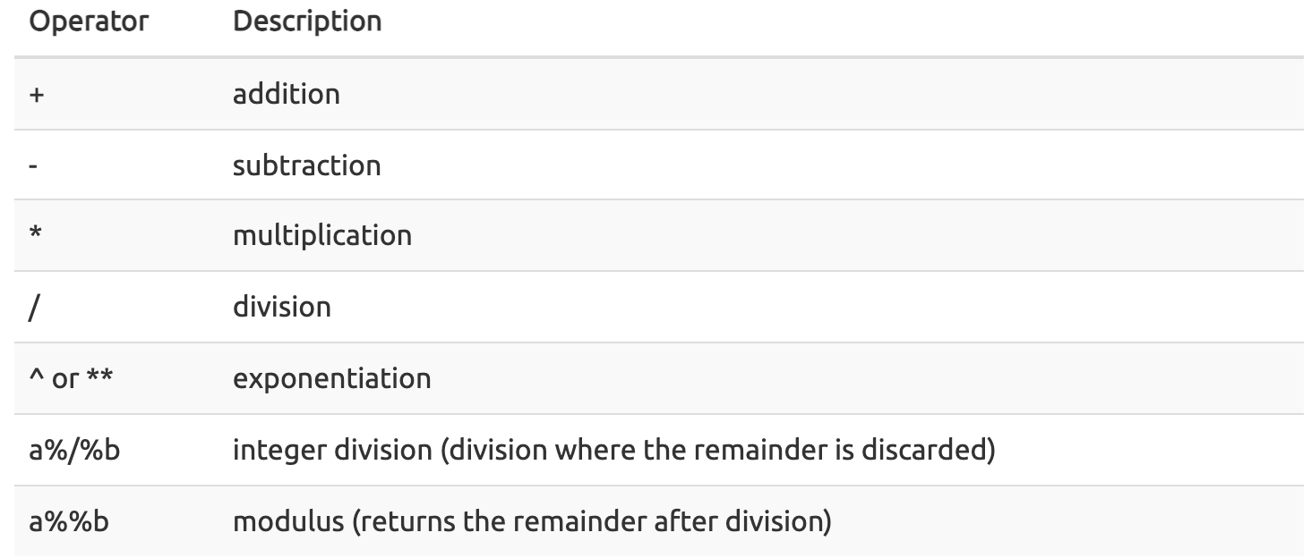
() are additionally used to establish the order of operations.

Let's see this in practice.

#create an object storing the number of human chromosomes (haploid)
human_chr_number<-23
#let's check the mode of this object
mode(human_chr_number)

[1] "numeric"

#Now, lets get the total number of human chromosomes (diploid)
human_chr_number * 2 #The output is 46! 

[1] 46

Moreover, we do not need an object to perform mathematical computations. R can be used like a calculator.

For example,

(1 + (5^0.5))/2

[1] 1.618034

A function is an object.

R functions are saved as objects, and if we type the name of the function, we can see the value of the object (i.e., the code underlying the function). Functions are important to R programming, as anything that happens in R is due to the use of a function.

We have used some R functions in Lesson 1 (e.g. getwd() and setwd())! Let's look at another example using the round() function.
round() "rounds the values in its first argument to the specified number of decimal places (default 0)" --- R help.

Consider

round(5.65) #can provide a single number

[1] 6

round(c(5.65,7.68,8.23)) #can provide a vector

[1] 6 8 8

In this example, we only provided the required argument in this case, which was any numeric or complex vector. We can see that two arguments can be included by the context prompt while typing (See below image). The optional second argument (i.e., digits) indicates the number of decimal places to round to. Contextual help is generally provided as you type the name of a function in RStudio.

#provide an additional argument rounding to the tenths place
round(5.65,digits=1) 

[1] 5.7

At times a function may be masked by another function. This can happen if two functions are named the same (e.g., dplyr::filter() vs plyr::filter()). We can get around this by explicitly calling a function from the correct package using the following syntax: package::function().

The pipe (|>, %>%)

Functions can be chained together using a pipe.

• |> is the native base R pipe, introduced in R 4.1.0 (2021).
• %>% is the pipe from the magrittr package (commonly used in the tidyverse).

For new learners, it is recommended to use the native pipe |> unless working within tidyverse-heavy workflows. The pipe improves readability by minimizing nested function calls.

For example,

ex<- -5.679

abs(round(ex)) # nested

[1] 6

ex |> round() |> abs() # Using the pipe

[1] 6

We will talk about the pipe more in part 2 and 3 of this series. For now, it is helpful to know that it exists and what it is doing.

Pre-defined objects

Base R comes with a number of built-in functions, vectors, data frames, and other objects. You can view built-in primitive functions and core base R functions with builtins(). You can view built-in datasets using data(). To explore datasets included with base R use help(package = "datasets").

Test your learning

Given the following R code:

numbers<- c("1","2.56","83","678")

What type of data is stored in this vector?
a. double
b. character
c. logical
d. complex

Which of the following are valid names for R objects? Select all that apply.

.3f <- 7

.fff <- 7

$%^ <- 7

This? <- 7

this.one <- 7

this_one <- 7

.fff <- 7  

this.one <- 7

this_one <- 7

Acknowledgments

Material from this lesson was either taken directly or adapted from the Intro to R and RStudio for Genomics lesson provided by Data Carpentry.