Multimodal Spatial Transcriptomic Characterization of Mouse Kidney Injury and Repair
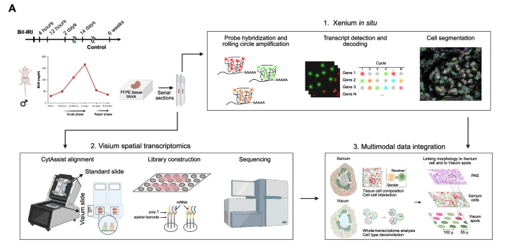
This study was designed to understand how acute kidney injury (AKI) progresses toward chronic kidney disease (CKD) by examining both the spatial organization and molecular programs of cells during injury and repair. Using a mouse model of bilateral ischemia–reperfusion injury, kidneys were collected at multiple time points (immediately after sham surgery, 4 Hours, 12 Hours, 2 Days, 14 Days, and 6 Week post surgery) spanning early injury to late fibrosis.
-
The authors combined two complementary spatial transcriptomics platforms on adjacent tissue sections: Xenium, an imaging-based method that provides single-cell resolution but measures a targeted gene panel, and Visium, a sequencing-based method that captures whole-transcriptome data at lower spatial resolution.
-
By integrating these datasets, they first defined distinct cell types and spatial “neighborhoods” at single-cell resolution using Xenium, and then projected these neighborhoods onto the Visium data to characterize their broader gene expression programs, signaling pathways, and transcription factor activities. This multimodal approach allowed them to identify a fibro-inflammatory niche enriched in failed-repair proximal tubule cells, fibroblasts, and immune cells, and to infer molecular mechanisms—such as PDGF and integrin signaling—that may drive maladaptive repair and fibrosis following AKI.
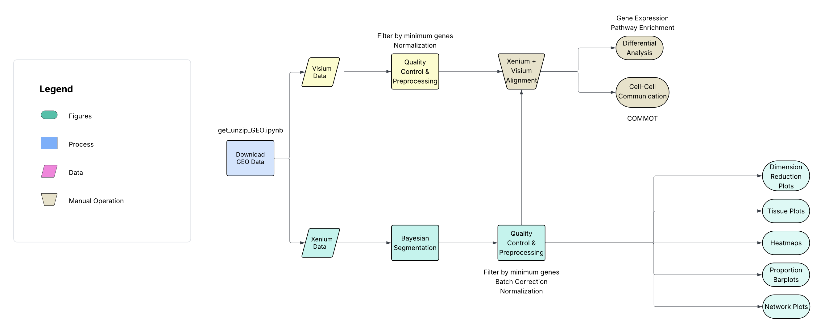
The bioinformatics workflow for this study can be represented by the following diagram:
Get the Data
The multimodal spatial data bundle is available here: MultimodalSpatial.zip.
This zip file contains the pre-processed Xenium AnnData object (Xenium_all.h5ad), the pre-processed Visium AnnData object (visium_fullres_all.h5ad), and the companion notebook for downloading and unpacking the GEO source data (get_unzip_GEO.ipynb).
Loading Python Packages for Spatial Transcriptomics
Python is the primary language used by the authors for spatial transcriptomic analysis due to its efficient memory management and strong support for handling large, multi-modal datasets.
The main libaries that will be used are Anndata, Scanpy, and Squidpy. Gene expression matrices and associated metadata are stored within an AnnData object. Standard workflows for quality control, normalization, clustering, dimensionality reduction, and differential expression analysis are implemented using the Scanpy library.
The Squidpy package provides specialized methods for spatial transcriptomic analysis, including visualization of spatial neighborhoods, spatial graph construction, and graph-based analytical approaches.
# -----------------------------
# Standard library
# -----------------------------
import os
import sys
import glob
import math

# -----------------------------
# Core scientific Python stack
# -----------------------------
import numpy as np
import pandas as pd
import matplotlib.pyplot as plt

# -----------------------------
# Single-cell / spatial omics
# -----------------------------
import anndata as ad
import commot as ct
import scanpy as sc
import scanpy.external as sce
import squidpy as sq
import pySTIM as pst
from gseapy import barplot, dotplot

# -----------------------------
# SpatialData / Xenium I/O
# -----------------------------
from spatialdata_io import xenium
from spatialdata.models import TableModel, ShapesModel

# -----------------------------
# Geo / shapes
# -----------------------------
import geopandas as gpd
from shapely.geometry import Polygon

# -----------------------------
# ML / sparse / graphs
# -----------------------------
import networkx as nx
from scipy.sparse import csr_matrix, coo_matrix
from sklearn.neighbors import radius_neighbors_graph

# -----------------------------
# Stats
# -----------------------------
from scipy.stats import norm
from statsmodels.stats.multitest import multipletests

# -----------------------------
# Batch correction / integration
# -----------------------------
import harmonypy as hm

# -----------------------------
# Plotting helpers
# -----------------------------
import seaborn as sns
import matplotlib.colors as mcolors
import matplotlib.cm as cm
import matplotlib.patches as mpatches
from matplotlib.collections import PolyCollection
from matplotlib.colors import to_hex, to_rgba
from matplotlib.legend_handler import HandlerPatch
from matplotlib.pyplot import rc_context

# Clear warnings for cleaner presentation
import warnings
warnings.filterwarnings('ignore')
Important
Before running the code for Section I: Loading Files and Pre-processing, download the files from Get the Data. The bundle includes get_unzip_GEO.ipynb for retrieving and unpacking the GEO source data.
Section I: Loading Files and Pre-processing
Warning
This section can be computationally intensive. To save time, skip to Section II: Preliminary Analysis, which uses the pre-processed h5ad files listed in Get the Data.
Loading Xenium files from 10x
10x Xenium data are typically organized into a structured output folder containing:
-
raw and processed microscopy images (e.g., OME-TIFF)
-
transcript-level tables listing each detected molecule with gene identity and spatial coordinates (x, y, sometimes z)
-
cell-level metadata including cell IDs, segmentation polygons, centroids, and gene count matrices
-
experiment-level summary files and QC metrics.
The following code extracts the Xenium files downloaded from the GEO repository: GSE269719. For each of the six tissue samples (sham, Hour2, Hour12, Day2, Day14, Week6), the slide image (1), transcript data (2), and metadata (3) are stored inside an anndata object. The anndata objects are organized inside a dictionary for downstream sample-based filtering and normalization.
base_dir = "./Input/Xenium"

# list only subdirectories
xenium_dirs = [
    d for d in os.listdir(base_dir)
    if os.path.isdir(os.path.join(base_dir, d))
]

xenium_dict = {}

for d in xenium_dirs:
    xenium_path = os.path.join(base_dir, d)

    # key like "Day14L" from "Day14L-output-..."
    key = d.split("-output")[0]

    # read Xenium dataset
    adata = xenium(xenium_path)
    xenium_dict[key] = adata
[33mWARNING [0m The `feature_key` column feature_name is categorical with unknown categories. Please ensure the categories
are known before calling `[1;35mPointsModel.parse[0m[1m([0m[1m)[0m` to avoid significant performance implications due to the
need for dask to compute the categories. If you did not use [1;35mPointsModel.parse[0m[1m([0m[1m)[0m explicitly in your code
[1m([0me.g. this message is coming from a reader in `spatialdata_io`[1m)[0m, please report this finding.
Baysor Segmentation
By default, Xenium provides a nucleus- or morphology-based segmentation that assigns transcripts to cells using image-derived boundaries. However, a drawback with this approach is that it might not delineate boundaries in dense or morphologically ambiguous regions.
The authors aim to improve boundary resolution by employing Baysor segmentation, which uses a Bayesian spatial model that incorporates both transcript density and gene identity patterns to probabilistically reassign molecules and redefine cell boundaries.
Demo:
https://kharchenkolab.github.io/Baysor/dev/.
Paper:
BAYSOR_ROOT = "./Input/Baysor"

for sample, sdata in xenium_dict.items():
    bdir = os.path.join(BAYSOR_ROOT, sample)
    if not os.path.isdir(bdir):
        print(f"[skip] no Baysor folder for {sample}")
        continue

    # --- 1) Baysor polygons -> shapes ---
    poly = pd.read_csv(os.path.join(bdir, "polygon.csv"))  # polygon_number, x_location, y_location

    polys = (
        poly.groupby("polygon_number")[["x_location", "y_location"]]
            .apply(lambda df: Polygon(df.to_numpy()))
    )

    gdf = gpd.GeoDataFrame(
        {"baysor_cell_id": polys.index.astype(str)},
        geometry=polys.values,
    ).set_index("baysor_cell_id")

    # IMPORTANT: parse to add required SpatialData metadata (transform, etc.)
    sdata.shapes["baysor_cell_boundaries"] = ShapesModel.parse(gdf)

    # --- 2) Baysor counts -> AnnData table (cell x gene) ---
    counts = pd.read_csv(os.path.join(bdir, "segmentation_counts.tsv"), sep="\t").set_index("gene").T
    counts.index = counts.index.astype(str)

    adata_b = ad.AnnData(X=counts.values)
    adata_b.obs_names = counts.index
    adata_b.var_names = counts.columns.astype(str)

    sdata.tables["baysor_table"] = TableModel.parse(adata_b)

    seg = pd.read_csv(os.path.join(bdir, "segmentation.csv"), usecols=["transcript_id", "cell_id"])
    seg["cell_id"] = seg["cell_id"].astype(str)

    # Make an AnnData where each row = one transcript
    seg_adata = ad.AnnData(X=np.zeros((len(seg), 0), dtype=np.float32))
    seg_adata.obs = seg.set_index("transcript_id")  # transcript_id as index, cell_id in obs

    sdata.tables["baysor_transcript_map"] = TableModel.parse(seg_adata)
/home/bianjh/.conda/envs/BTEP_spat/lib/python3.12/functools.py:912: ImplicitModificationWarning: Transforming to str index.
  return dispatch(args[0].__class__)(*args, **kw)


[ok] updated Day14L


/home/bianjh/.conda/envs/BTEP_spat/lib/python3.12/functools.py:912: ImplicitModificationWarning: Transforming to str index.
  return dispatch(args[0].__class__)(*args, **kw)


[ok] updated Day14R


/home/bianjh/.conda/envs/BTEP_spat/lib/python3.12/functools.py:912: ImplicitModificationWarning: Transforming to str index.
  return dispatch(args[0].__class__)(*args, **kw)


[ok] updated Day2L


/home/bianjh/.conda/envs/BTEP_spat/lib/python3.12/functools.py:912: ImplicitModificationWarning: Transforming to str index.
  return dispatch(args[0].__class__)(*args, **kw)


[ok] updated Day2R


/home/bianjh/.conda/envs/BTEP_spat/lib/python3.12/functools.py:912: ImplicitModificationWarning: Transforming to str index.
  return dispatch(args[0].__class__)(*args, **kw)


[ok] updated Hour12L


/home/bianjh/.conda/envs/BTEP_spat/lib/python3.12/functools.py:912: ImplicitModificationWarning: Transforming to str index.
  return dispatch(args[0].__class__)(*args, **kw)


[ok] updated Hour12R


/home/bianjh/.conda/envs/BTEP_spat/lib/python3.12/functools.py:912: ImplicitModificationWarning: Transforming to str index.
  return dispatch(args[0].__class__)(*args, **kw)


[ok] updated Hour4L


/home/bianjh/.conda/envs/BTEP_spat/lib/python3.12/functools.py:912: ImplicitModificationWarning: Transforming to str index.
  return dispatch(args[0].__class__)(*args, **kw)


[ok] updated Hour4R


/home/bianjh/.conda/envs/BTEP_spat/lib/python3.12/functools.py:912: ImplicitModificationWarning: Transforming to str index.
  return dispatch(args[0].__class__)(*args, **kw)


[ok] updated ShamL


/home/bianjh/.conda/envs/BTEP_spat/lib/python3.12/functools.py:912: ImplicitModificationWarning: Transforming to str index.
  return dispatch(args[0].__class__)(*args, **kw)


[ok] updated ShamR


/home/bianjh/.conda/envs/BTEP_spat/lib/python3.12/functools.py:912: ImplicitModificationWarning: Transforming to str index.
  return dispatch(args[0].__class__)(*args, **kw)


[ok] updated Week6L


/home/bianjh/.conda/envs/BTEP_spat/lib/python3.12/functools.py:912: ImplicitModificationWarning: Transforming to str index.
  return dispatch(args[0].__class__)(*args, **kw)


[ok] updated Week6R
Save segmented data as zarr files
zarr files are generally used to store xenium data. For each of the above samples, it is recommended to save the segmented data as backup copies. The python package spatialdata is used to read and manage zarr files.
Check to ensure that the following information are present:
- Images
- Shapes (polygons)
- Points (transcripts)
- Tables (AnnData)
- Labels
for sample, sdata in xenium_dict.items():
    sdata.write(f"./Output/{sample}.zarr")
# check that zarr file can be read
from spatialdata import read_zarr

spadata_dict = {}

for fname in os.listdir("./Output"):
    if not fname.endswith(".zarr"):
        continue
    sample = fname.replace(".zarr", "")
    if sample in ["ShamR", "Hour4R", "Hour12R"]:
        sdata = read_zarr(os.path.join("./Output", fname))
        spadata_dict[sample] = sdata.tables["table"].copy()  # AnnData
Filtering and Normalization
For each sample, filter out tissue spots containing fewer than 3 genes and 10 Unique Molecular Identifiers (UMIs). Next, we merge the filtered samples, perform log normalization on the transcript expression data. Then, we run Principal Component Analysis, which is a required step for downstream UMAP / tSNE visualization, clustering, and harmony batch correction.
# 1) per-sample filter + label
for key, a in spadata_dict.items():
    sc.pp.filter_cells(a, min_genes=3)
    sc.pp.filter_cells(a, min_counts=10)

    a.obs_names = [f"{key}_{i}" for i in a.obs_names]
    a.obs["ident"] = key

# 2) concat
kidney_all = ad.concat(list(spadata_dict.values()), join="inner", label="ident", keys=spadata_dict.keys())
kidney_all.obs["ident"] = kidney_all.obs["ident"].astype("category")

# (optional) preserve raw counts
kidney_all.raw = kidney_all.copy()

# 3) normalize + log1p
sc.pp.normalize_total(kidney_all, target_sum=100)
sc.pp.log1p(kidney_all)

# 4) PCA
sc.pp.pca(kidney_all)
Batch Correction
If tissues were processed and sequenced on different days, it is possible that cluster separations in downstream steps can be attributed to batch differences. To help ensure that the variations we see in PCA, UMAPs, and tSNEs are due to biology and not technical effects such as date of sequencing, we employ Harmony batch correction.
https://portals.broadinstitute.org/harmony/articles/quickstart.html
# Run Harmony (batch key = ident)
ho = hm.run_harmony(X, kidney_all.obs, vars_use=["ident"], max_iter_harmony=15)

# Z_corr is (n_pcs, n_cells) in harmonypy -> transpose to (n_cells, n_pcs)
X_harmony = ho.Z_corr

kidney_all.obsm["X_pca_harmony"] = X_harmony
2026-02-21 12:22:51,746 - harmonypy - INFO - Running Harmony (PyTorch on cpu)
2026-02-21 12:22:51,747 - harmonypy - INFO -   Parameters:
2026-02-21 12:22:51,747 - harmonypy - INFO -     max_iter_harmony: 15
2026-02-21 12:22:51,747 - harmonypy - INFO -     max_iter_kmeans: 20
2026-02-21 12:22:51,747 - harmonypy - INFO -     epsilon_cluster: 1e-05
2026-02-21 12:22:51,748 - harmonypy - INFO -     epsilon_harmony: 0.0001
2026-02-21 12:22:51,748 - harmonypy - INFO -     nclust: 100
2026-02-21 12:22:51,748 - harmonypy - INFO -     block_size: 0.05
2026-02-21 12:22:51,748 - harmonypy - INFO -     lamb: [1. 1. 1.]
2026-02-21 12:22:51,749 - harmonypy - INFO -     theta: [2. 2. 2.]
2026-02-21 12:22:51,749 - harmonypy - INFO -     sigma: [0.1 0.1 0.1 0.1 0.1]...
2026-02-21 12:22:51,749 - harmonypy - INFO -     verbose: True
2026-02-21 12:22:51,750 - harmonypy - INFO -     random_state: 0
2026-02-21 12:22:51,750 - harmonypy - INFO -   Data: 50 PCs × 309712 cells
2026-02-21 12:22:51,750 - harmonypy - INFO -   Batch variables: ['ident']
2026-02-21 12:22:51,873 - harmonypy - INFO - Computing initial centroids with sklearn.KMeans...
2026-02-21 12:22:56,453 - harmonypy - INFO - KMeans initialization complete.
2026-02-21 12:22:56,974 - harmonypy - INFO - Iteration 1 of 15
2026-02-21 12:23:26,840 - harmonypy - INFO - Iteration 2 of 15
2026-02-21 12:23:56,513 - harmonypy - INFO - Iteration 3 of 15
2026-02-21 12:24:25,869 - harmonypy - INFO - Iteration 4 of 15
2026-02-21 12:24:55,518 - harmonypy - INFO - Iteration 5 of 15
2026-02-21 12:25:25,079 - harmonypy - INFO - Iteration 6 of 15
2026-02-21 12:25:52,096 - harmonypy - INFO - Iteration 7 of 15
2026-02-21 12:26:07,082 - harmonypy - INFO - Iteration 8 of 15
2026-02-21 12:26:20,560 - harmonypy - INFO - Iteration 9 of 15
2026-02-21 12:26:35,056 - harmonypy - INFO - Converged after 9 iterations
Cell Type Annotation
Celltypes were annotated via snRNA Integration (R-Seurat Query Mapping). For the purpose of this demo, we will use a version of the anndata that has been already annotated by the authors (Xenium_all.h5ad).
Loading Visium Data from 10x
10x Visium data are organized into a Space Ranger output directory containing both gene expression matrices and spatial metadata. Key components include:
-
a filtered and raw feature-barcode matrix (MTX, H5, or CSV formats) with gene counts per spot
-
a spatial/ folder containing high-resolution and low-resolution tissue images
-
a tissue_positions.csv (or parquet) file listing each spot barcode with its array coordinates and pixel positions on the image
-
a scalefactors_json.json file used to map spot coordinates to image space
-
summary QC and web summary reports.
Unlike Xenium, Visium data are spot-based rather than single-cell resolved, with each spot (∼55 µm diameter in v1 chemistry) capturing transcripts from multiple cells, making downstream analyses dependent on deconvolution or integration methods to infer cell-type composition.
The following code loads the visium data for each of the six samples.
sham = sc.read_visium(path = '/vf/users/CCBR/jingIODC/BTEP_Xenium_Visium/Input/mouse_data/mouse_sham/outs/')
hour4 = sc.read_visium(path = '/vf/users/CCBR/jingIODC/BTEP_Xenium_Visium/Input/mouse_data/mouse_hour4/outs/')
hour12 = sc.read_visium(path = '/vf/users/CCBR/jingIODC/BTEP_Xenium_Visium/Input/mouse_data/mouse_hour12/outs/')
day2 = sc.read_visium(path = '/vf/users/CCBR/jingIODC/BTEP_Xenium_Visium/Input/mouse_data/mouse_day2/outs/')
day14 = sc.read_visium(path = '/vf/users/CCBR/jingIODC/BTEP_Xenium_Visium/Input/mouse_data/mouse_day14/outs/')
week6 = sc.read_visium(path = '/vf/users/CCBR/jingIODC/BTEP_Xenium_Visium/Input/mouse_data/mouse_week6/outs/')
Similar to the pre-processing steps for Xenium data, we perform filtering and quality control for each individual tissue sample. After this, we merge the pre-processed samples into one adata object, perform log-normalization, select top variable genes, and perform Principal Component Analysis (PCA).
ad_list = [sham,hour4,hour12,day2,day14,week6]

# be sure to append sample name to metadata column, to know which spot comes from which sample
for item in ad_list:
    item.var_names_make_unique()
    sc.pp.filter_cells(item, min_counts = 500)
    item.obs["spot_id"] = item.obs_names
    item.obsm["spatial"] = item.obsm["spatial"].astype(int)

for item in ad_list:
    sc.pp.calculate_qc_metrics(item, inplace=True)
    item.var['mt'] = [gene.startswith('MT-') for gene in item.var_names]
    item.obs['mt_frac'] = item[:, item.var['mt']].X.sum(1).A.squeeze()/item.obs['total_counts']


for item in ad_list:
    item.obs["X_coords"] = item.obsm["spatial"][:,0]
    item.obs["Y_coords"] = item.obsm["spatial"][:,1]
sample_names = ["ShamR", "Hour4R", "Hour12R", "Day2R", "Day14R", "Week6R"]

for a, name in zip(ad_list, sample_names):
    a.obs_names = [f"{name}_{bc}" for bc in a.obs_names]

adata = ad.concat(
    ad_list,
    join="inner",
    label="ident",
    keys=sample_names,
    fill_value=0,
    uns_merge="unique"
)

adata.raw = adata

sc.pp.normalize_total(adata, inplace = True)
sc.pp.log1p(adata)
sc.pp.highly_variable_genes(adata, flavor='seurat', n_top_genes=3000, inplace=True)

sc.pp.pca(adata)
X = adata.obsm["X_pca"]
# ensure a plain numpy array (and 2D)
X = np.asarray(X)
if X.ndim != 2:
    raise ValueError(f"X_pca is not 2D, got {X.shape}")

ho = hm.run_harmony(X, adata.obs, "ident", max_iter_harmony=15)

Z = ho.Z_corr  # often (n_pcs, n_cells)
Z = np.asarray(Z)

# Make it cells × PCs no matter what orientation harmonypy returned
if Z.shape[0] == adata.n_obs:
    X_harmony = Z
elif Z.shape[1] == adata.n_obs:
    X_harmony = Z.T
else:
    raise ValueError(f"Unexpected Z_corr shape {Z.shape} for n_obs={adata.n_obs}")

adata.obsm["X_pca_harmony"] = X_harmony

adata.obsm["X_pca"] = adata.obsm["X_pca_harmony"]
2026-02-25 16:39:35,086 - harmonypy - INFO - Running Harmony (PyTorch on cpu)
2026-02-25 16:39:35,088 - harmonypy - INFO -   Parameters:
2026-02-25 16:39:35,090 - harmonypy - INFO -     max_iter_harmony: 15
2026-02-25 16:39:35,093 - harmonypy - INFO -     max_iter_kmeans: 20
2026-02-25 16:39:35,095 - harmonypy - INFO -     epsilon_cluster: 1e-05
2026-02-25 16:39:35,097 - harmonypy - INFO -     epsilon_harmony: 0.0001
2026-02-25 16:39:35,099 - harmonypy - INFO -     nclust: 100
2026-02-25 16:39:35,101 - harmonypy - INFO -     block_size: 0.05
2026-02-25 16:39:35,103 - harmonypy - INFO -     lamb: [1. 1. 1. 1. 1. 1.]
2026-02-25 16:39:35,106 - harmonypy - INFO -     theta: [2. 2. 2. 2. 2. 2.]
2026-02-25 16:39:35,108 - harmonypy - INFO -     sigma: [0.1 0.1 0.1 0.1 0.1]...
2026-02-25 16:39:35,110 - harmonypy - INFO -     verbose: True
2026-02-25 16:39:35,112 - harmonypy - INFO -     random_state: 0
2026-02-25 16:39:35,114 - harmonypy - INFO -   Data: 50 PCs × 19432 cells
2026-02-25 16:39:35,116 - harmonypy - INFO -   Batch variables: ['ident']
2026-02-25 16:39:35,228 - harmonypy - INFO - Computing initial centroids with sklearn.KMeans...
2026-02-25 16:39:36,395 - harmonypy - INFO - KMeans initialization complete.
2026-02-25 16:39:36,485 - harmonypy - INFO - Iteration 1 of 15
2026-02-25 16:39:46,530 - harmonypy - INFO - Iteration 2 of 15
2026-02-25 16:39:56,349 - harmonypy - INFO - Iteration 3 of 15
2026-02-25 16:40:06,463 - harmonypy - INFO - Iteration 4 of 15
2026-02-25 16:40:16,232 - harmonypy - INFO - Iteration 5 of 15
2026-02-25 16:40:29,276 - harmonypy - INFO - Converged after 5 iterations
Create umap, run clustering, and save data as h5ad for downstream steps.
sc.pp.neighbors(adata, n_pcs=50)
sc.tl.umap(adata)

sc.tl.leiden(adata, resolution=2, key_added="res2")

adata.write("visium_fullres_all.h5ad")
/tmp/ipykernel_1371946/2948835038.py:4: FutureWarning: The `igraph` implementation of leiden clustering is *orders of magnitude faster*. Set the flavor argument to (and install if needed) 'igraph' to use it.
In the future, the default backend for leiden will be igraph instead of leidenalg. To achieve the future defaults please pass: `flavor='igraph'` and `n_iterations=2`. `directed` must also be `False` to work with igraph’s implementation.
  sc.tl.leiden(adata, resolution=2, key_added="res2")
Download visium_fullres_all.h5ad
The above code will save the pre-processed visium data as an h5ad file. You can download the bundled copy from Get the Data (visium_fullres_all.h5ad). This file will be used in downstream steps.
Section II. Preliminary Analyses
Xenium Preliminary Figures
Initial visualization of Xenium data focuses on spatial tissue plots in which transcript abundance for selected marker genes is overlaid directly onto the tissue coordinates. Each detected molecule is mapped to its spatial (x, y) position, and expression levels are visualized either at the transcript or cell-aggregated level using continuous color scales.
# set working directory to location containing processed h5ad data
os.chdir("path/to/dir/Xenium_all.h5ad")
adata = sc.read_h5ad("Xenium_all.h5ad")
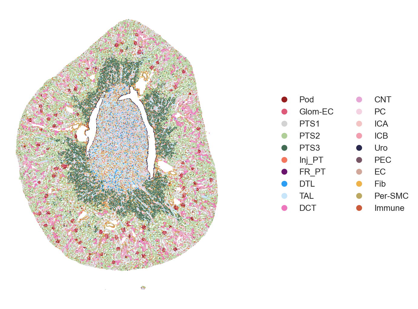
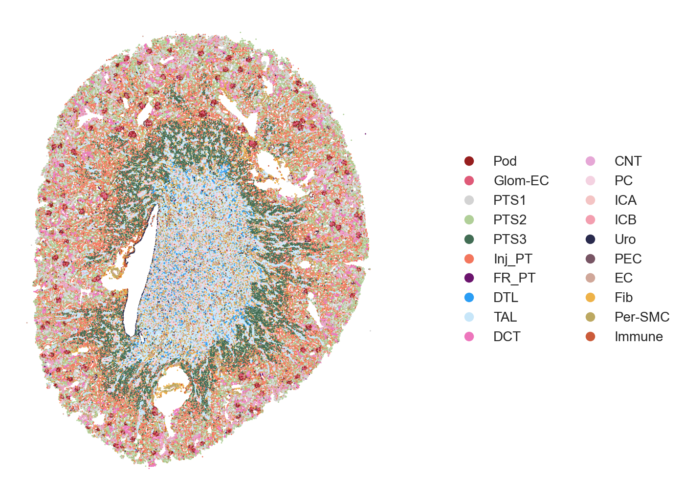
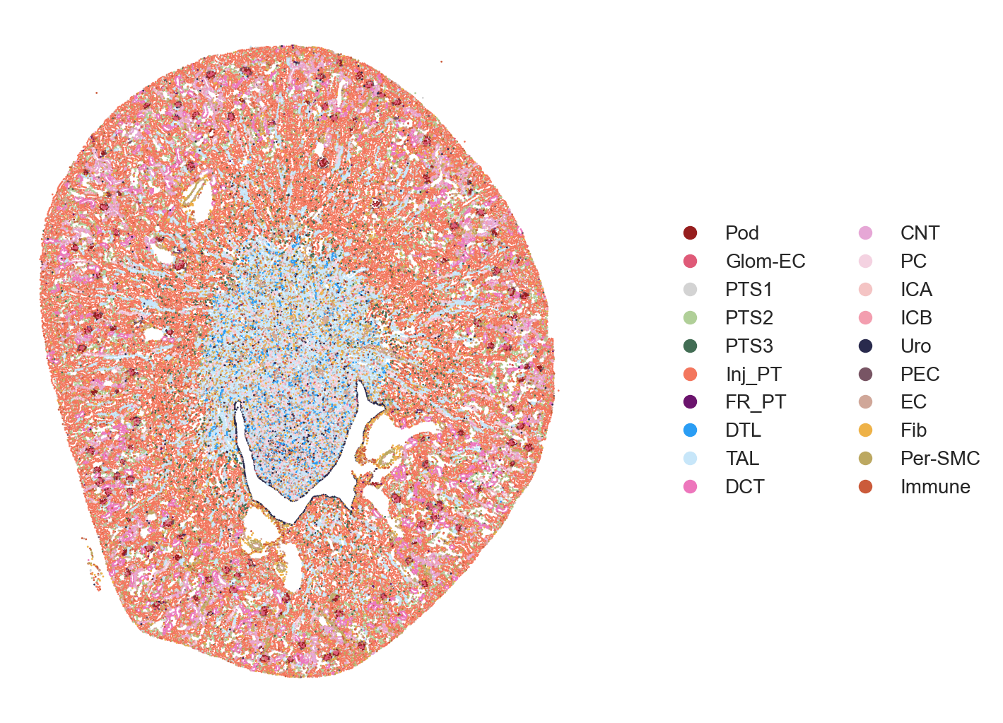
The authors visualized the spatiotemporal distribution of cell types within selected kidney regions, spanning from immediately after damage (Sham surgery) through AKI progression and repair time course. Full sections of the tissues can be visualized followed by specific subsections (e.g. cortex, medulla, etc.).
# Full Tissue Image
pst.plot_scatter(adata[adata.obs.ident == "ShamR"], dpi=200, ptsize=1,
                    color_by='celltype_plot', seed=123, alpha=1, ticks=False)
pst.plot_scatter(adata[adata.obs.ident == "Hour4R"], dpi=200, ptsize=1,
                    color_by='celltype_plot', seed=123, alpha=1, ticks=False)
pst.plot_scatter(adata[adata.obs.ident == "Hour12R"], dpi=200, ptsize=1,
                    color_by='celltype_plot', seed=123, alpha=1, ticks=False)
The area to visualize can be choosen using the xlims and ylims parameter in plot_scatter().
## Celltype Visualization - 2A (Sham, Hour4, Hour12)
pst.plot_scatter(adata[adata.obs.ident == "ShamR"], xlims=[1850,2150], ylims=[500,1400], dpi=200, ptsize=15,
                    color_by='celltype_plot', seed=123, alpha=1, ticks=False)
pst.plot_scatter(adata[adata.obs.ident == "Hour4R"], xlims=[2700,3000], ylims=[3200,4100], dpi=200, ptsize=15,
                    color_by='celltype_plot', seed=123, alpha=1, ticks=False)
pst.plot_scatter(adata[adata.obs.ident == "Hour12R"], xlims=[2300,2600], ylims=[1450,2350], dpi=200, ptsize=15,
                    color_by='celltype_plot', seed=123, alpha=1, ticks=False)
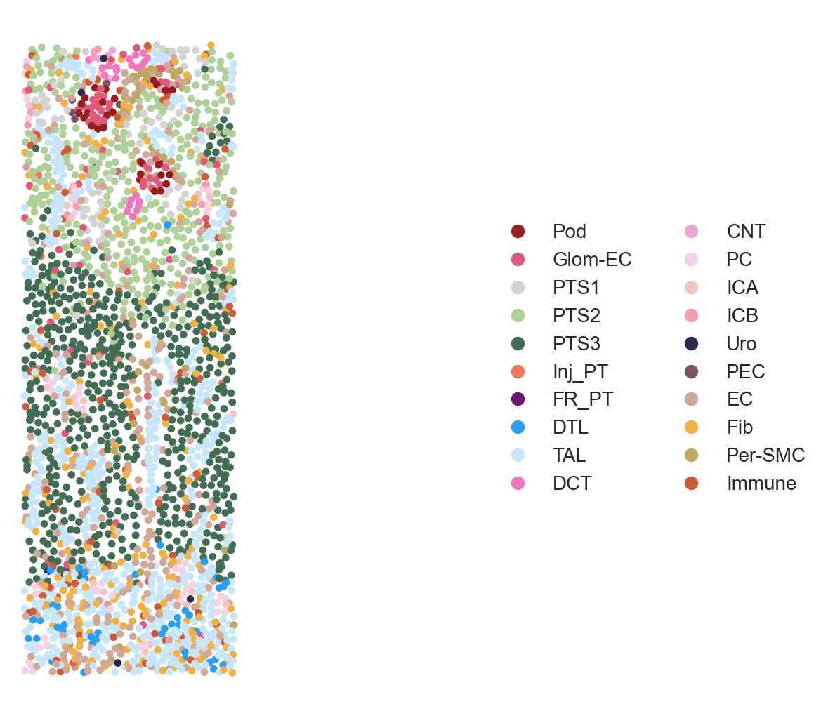
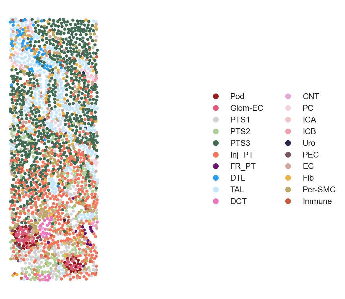
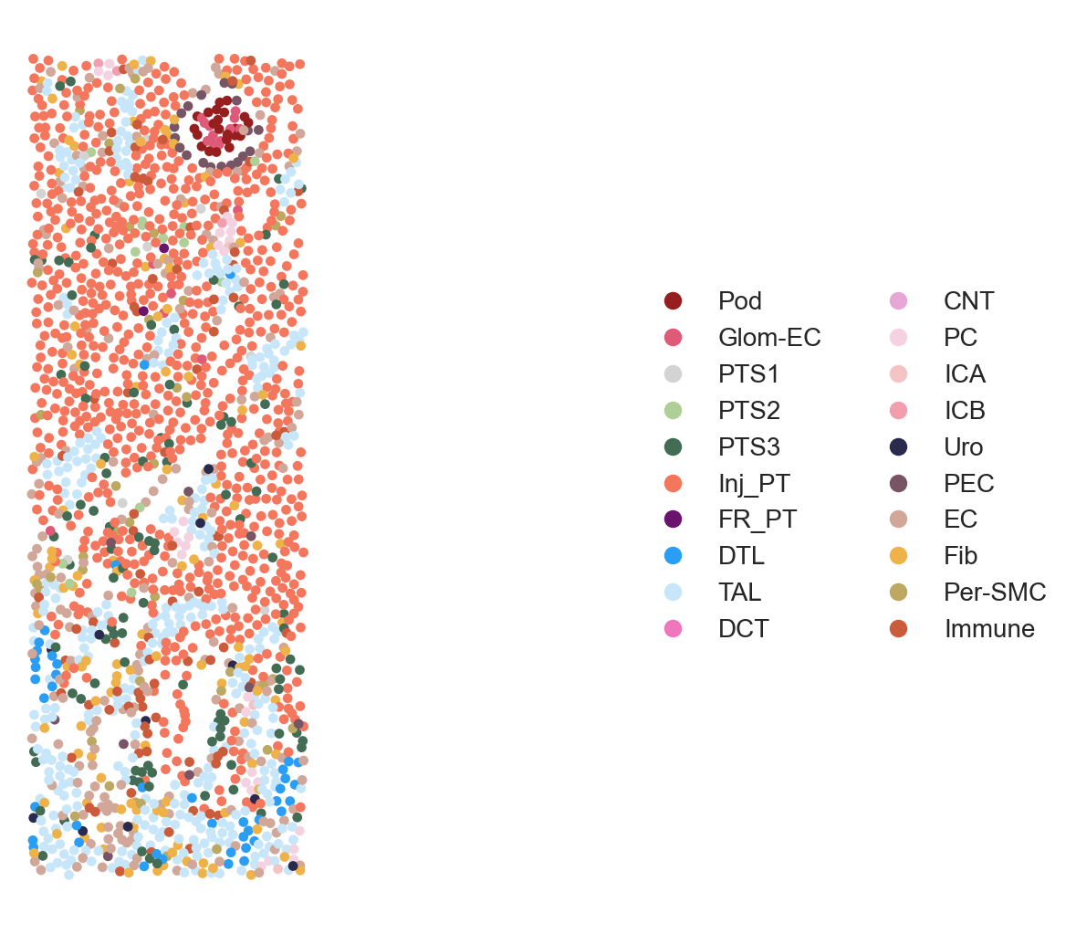
Figure 2A. Celltype Visualization
To summarize expression patterns across segmented cells, gene expression matrices were aggregated at the cell level and visualized using heatmaps. Typically, cells are grouped by cluster or annotation (e.g., cell type or niche), and scaled expression values highlight relative enrichment of canonical markers across groups. For Figure 2B, the authors visualized canonical markers across celltype-enriched spots across tissues.
# Figure 2B
genes = ['Nphs2','Ddn','Ehd3', 'Slc5a2', 'Slc5a12', 'Cyp4b1','Slc22a6', 'Slc7a13', 'Acox2', 'Cyp7b1', 'Plin2', "Krt20", 'Havcr1',
         'Vcam1', 'C3', 'Fst', 'Slc12a1', 'Slc12a3', 'Scnn1g',  'Aqp4',"Clnk",
         'Slc26a4', 'Krt19','Krt15', "Akap12",
         'Emcn', "Col1a1",'Fbln1','Cxcl12', 'Acta2', 'Myh11', 'Cd53','Ccl8','Ccr1']

adata.layers["scaled"] = sc.pp.scale(adata, copy=True).X

with rc_context({'figure.dpi': 300}):
    ax_dict = sc.pl.matrixplot(adata, genes, 'celltype_plot', dendrogram=False, figsize=(5,5), layer='scaled', swap_axes=True,
                               vmin=-1.5, vmax=1.5, cmap='RdBu_r', show=False)

    ax_dict['mainplot_ax'].tick_params(axis='both', which='both', length=0)
    ax_dict['color_legend_ax'].set_visible(False)
    plt.show()
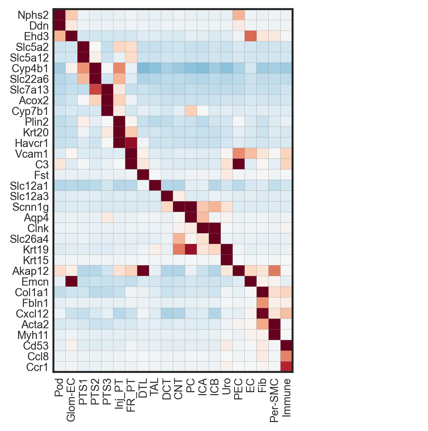
Figure 2B. Scaled expression of canonical marker genes across cell types.
Uniform Manifold Approximation and Projection (UMAP) is then used to embed high-dimensional cell-level expression profiles into a two-dimensional space, enabling visualization of transcriptional similarity among cells. Clusters emerging in UMAP space often correspond to distinct cell types or states and can be annotated using known marker genes (e.g. PTS1,PTS2,PTS3, and Inj_PT). When combined with spatial mapping, UMAP enables comparison between transcriptional neighborhoods and physical tissue organization, revealing whether molecularly similar cells are spatially clustered or dispersed.
# Figure 2C
with plt.rc_context({"figure.dpi": (200), "figure.figsize": (5,5)}):
    ax = sc.pl.umap(adata, color=["celltype_plot"], s=0.2,
                    legend_fontsize=4,
                    frameon=False,
                    show=False,legend_loc="on data")
    plt.show()
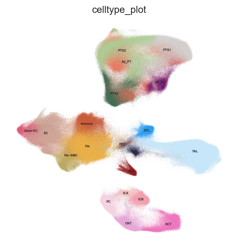
Figure 2C. UMAP embedding of single cells colored by cell type annotation.
Proportion Barplot of Celltype across Timepoints
From Figure 2A, it can visually observed that Inj_PT cells increased in numbers over the course of injury (Hour 2 and Hour 12). Cell counts and proportions can be quantified and tracked across timepoints with stacked barplots.
# Map each cell type to a color
categories = adata.obs["celltype_plot"].cat.categories
palette = plt.cm.tab20.colors[:len(categories)]

adata.uns["celltype_colors"] = [to_hex(c) for c in palette]
celltype_color_dict = dict(zip(categories, adata.uns["celltype_colors"]))

# Build a dataframe of cell-type counts across timepoints
conditions = ["Sham", "Hour4", "Hour12", "Day2", "Day14", "Week6"]
adata.obs["time"] = adata.obs["ident"].str[:-1]

ct_df = pd.DataFrame()
for t in conditions:
    df = adata[adata.obs["time"] == t].obs["celltype_plot"].value_counts()
    ct_df[t] = df

ct_df = ct_df.fillna(0)
# Convert to proportions within each timepoint
normed_df = ct_df.div(ct_df.sum(axis=0), axis=1)

# Reorder rows by category and assign colors
normed_df = normed_df.loc[categories]
colors = [celltype_color_dict[ct] for ct in normed_df.index]

# Simple stacked bar plot
fig, ax = plt.subplots(figsize=(6, 3.5), dpi=300)

bottom = np.zeros(len(normed_df.columns))
for i, celltype in enumerate(normed_df.index):
    values = normed_df.loc[celltype].values
    ax.bar(
        normed_df.columns,
        values,
        bottom=bottom,
        color=colors[i],
        edgecolor="black",
        linewidth=0.5,
        label=celltype,
    )
    bottom += values

ax.set_ylim(0, 1)
ax.set_ylabel("Proportion of cells")
ax.set_xlabel("Timepoint")
ax.spines["top"].set_visible(False)
ax.spines["right"].set_visible(False)
ax.legend(bbox_to_anchor=(1.02, 1), loc="upper left", frameon=False)
plt.xticks(rotation=0)
plt.tight_layout()
plt.show()
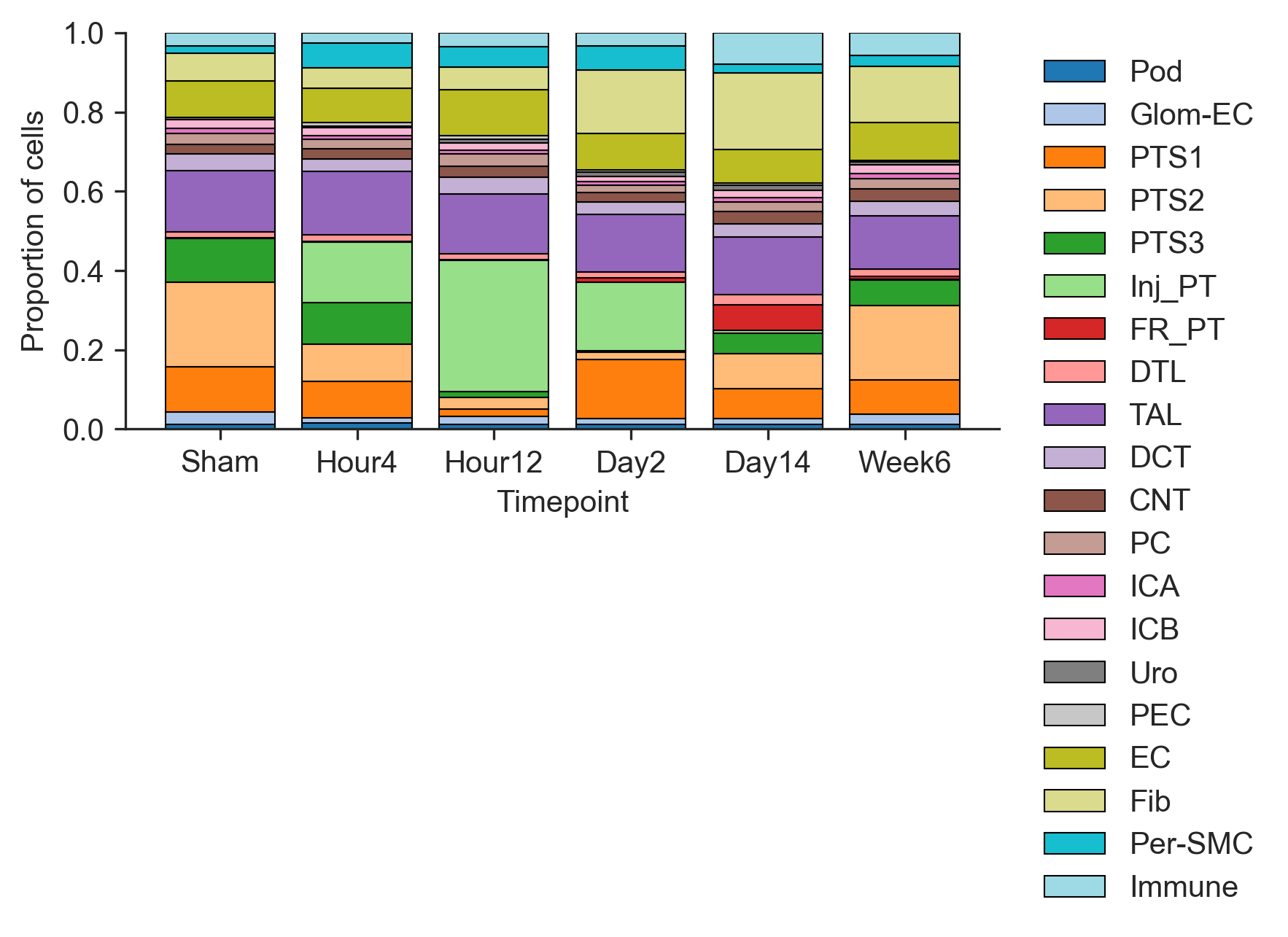
Injured PT proportion increased from Hour 4 to Hour 12, where it reaches its peak. The proportion of Injured PT then decreases towards Week 6. S2 segment of proximal tubule (PTS2) appears to follow an opposite trend; it decreases from Sham to Day2 before increasing again towards Week 6.
Gene Expression across Tissue Subregions Dotplot
In addition to proportion barplots, we can monitor gene expression across tissue subregions. A dot plot showing fraction of tissue spots enriched with genes commonly expressed over the course of injury and repair can be created using the following code.
genes = ['Slc5a12','Slc22a8', 'Cyp2e1','Slc7a13','Havcr1', 'Krt20', "C3", 'Cd74', 'Vcam1']
cmap = mcolors.LinearSegmentedColormap.from_list('WhRd',['#ffffff', "#fffacd", "red", "darkred"], N=256)
with plt.rc_context({"figure.dpi": (300)}):
    sc.pl.dotplot(adata, genes, 'CN', cmap = cmap, figsize=(5,2.5), show=False)
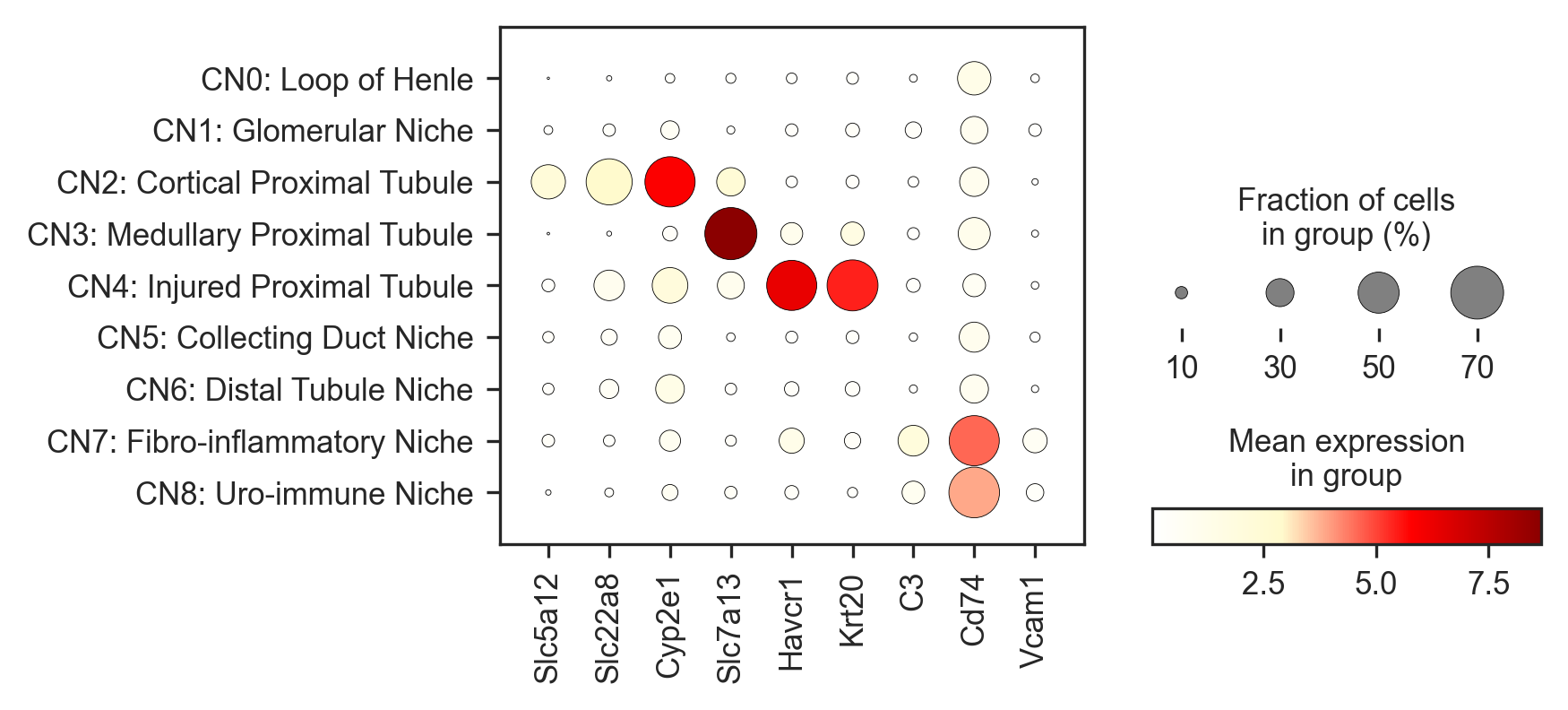
In the above figure, sodium transporter genes (Slc5a12, Slc22a8) were notibly expressed in low values within the Cortical Proximal Tubule across samples, while Cyp2e1, a marker of oxidative stress is highly expressed. Havcr1 and Krt20, markers of AKI injury and epithelium remodeling are notably expressed in high proportions and in mean expression within the Injured Proximal Tuble. Finally, Cd74 can be seen to be highly expressed in CN7 and CN8, neighborhoods association with immune activity and inflammation.
Spatial Permutation Analysis
To determine whether specific cell types are spatially enriched near one another, we performed a spatial permutation test. This approach evaluates whether observed cell–cell proximities are greater (or less) than expected by chance.
Overview
The method compares:
-
Observed spatial interactions between cell types
-
Expected interactions under random spatial organization
By generating a null distribution of interactions through spatial randomization, we can assess whether particular cell type pairs show statistically significant enrichment or depletion.
Step 1: Calculate Observed Cell–Cell Co-localization
Using the spatial coordinates of each cell, we identify neighboring cells within a defined niche radius (e.g., 15 µm). For every pair of neighboring cells:
-
We record their cell types.
-
We count how often each pair of cell types occurs in close proximity. This produces a matrix where:
Rows and columns represent cell types.
Each entry indicates how many neighboring pairs were observed between those two cell types.
The diagonal represents interactions between cells of the same type.
This matrix reflects the true spatial organization of the tissue.
Step 2: Generate a Null Model by Spatial Randomization
To determine whether the observed interactions are meaningful, we create a null model.
Instead of shuffling cell type labels, we randomly perturb (jitter) each cell’s spatial coordinates within a specified range (e.g., ±100 µm). This preserves:
- The total number of cells.
- The number of cells of each type
But disrupts their spatial relationships.
For each permutation:
-
Cell positions are randomly shifted.
-
Neighbor relationships are recalculated using the same niche radius.
-
Cell–cell interaction counts are recomputed.
This process is repeated many times (e.g., 100 permutations), generating a distribution of expected interaction counts under random spatial organization.
Step 3: Statistical Comparison
For each pair of cell types, we compare:
-
The observed number of neighboring interactions
-
The distribution of interaction counts from randomized data.
If the observed count is substantially higher than expected under random positioning, the pair is considered spatially enriched. If lower than expected, the pair may be spatially depleted.
def permute(adata, groupby = "celltype_raw",
            n_permutations = 100,
            niche_radius = 15.0,
            permute_radius = 100.0,
            spatial_key = "spatial",
            seed = 123):
    '''
    Permutation test: Randomizing the actual spatial locations of the cells, then computed the proximity
    between all possible pairs of cell types under this randomized spatial arrangement.
    '''
    categories_str_cat = list(adata.obs[groupby].cat.categories)
    categories_num_cat = range(len(categories_str_cat))
    map_dict = dict(zip(categories_num_cat, categories_str_cat))

    categories_str = adata.obs[groupby]
    categories_num = adata.obs[groupby].replace(categories_str_cat, categories_num_cat)
    labels = categories_num.to_numpy()
    print(len(labels))

    max_index = len(categories_num_cat)
    pair_counts = np.zeros((max_index, max_index))

    ## calculate the true interactions
    con = radius_neighbors_graph(adata.obsm[spatial_key], niche_radius,  mode='connectivity', include_self=False)
    con_coo = coo_matrix(con)
    print(f"Calculating observed interactions...")
    for i, j, val in zip(con_coo.row, con_coo.col, con_coo.data):
        if i >= j:
            continue

        type1 = labels[i]
        type2 = labels[j]

        if val:
            if type1 != type2:
                pair_counts[type1, type2] += 1
                pair_counts[type2, type1] += 1
            else:
                pair_counts[type1, type2] += 1

    #pair_counts = pair_counts/pair_counts.sum()  ## normalize by total counts
    ## calculate the null hypothesis
    coords = adata.obsm[spatial_key]

    pair_counts_null = np.zeros((max_index, max_index, n_permutations))

    for perm in range(n_permutations):
        np.random.seed(seed=None if seed is None else seed + perm)

        permuted_coords = coords + np.random.uniform(-permute_radius, permute_radius, size=coords.shape)
        permuted_con = radius_neighbors_graph(permuted_coords, niche_radius, mode='connectivity', include_self=False)
        permuted_con_coo = coo_matrix(permuted_con)

        if perm%100==1:
            print(f"Performing permutation {perm}...")

        pair_counts_permuted = np.zeros((max_index, max_index))

        for i, j, val in zip(permuted_con_coo.row, permuted_con_coo.col, permuted_con_coo.data):
            if i >= j:
                continue

            type1 = labels[i]
            type2 = labels[j]

            if val:
                if type1 != type2:
                    pair_counts_permuted[type1, type2] += 1
                    pair_counts_permuted[type2, type1] += 1
                else:
                    pair_counts_permuted[type1, type2] += 1

        #pair_counts_permuted = pair_counts_permuted/pair_counts_permuted.sum()  ## normalize by total counts
        pair_counts_null[:, :, perm] = pair_counts_permuted

    return categories_str_cat, pair_counts, pair_counts_null
for ident in adata.obs['ident'].unique():
    ad_perm = adata[adata.obs["ident"] == ident].copy()
    cell_cnt = pd.DataFrame(ad_perm.obs["celltype_plot"].value_counts()).reset_index()
    cell_cnt.columns = ['CellType', "Count"]

    celltypes, pair_counts, pair_counts_null = permute(ad_perm, "celltype_plot", n_permutations = 100,
                                                       niche_radius = 27.5, permute_radius = 50)
    pair_counts_permuted_means = np.mean(pair_counts_null, axis=2)
    pair_counts_permuted_stds = np.std(pair_counts_null, axis=2)

    z_scores = (pair_counts - pair_counts_permuted_means) / pair_counts_permuted_stds
    z_scores[z_scores<0]=0
    z_score_df = pd.DataFrame(z_scores,index = celltypes, columns = celltypes)
    z_score_df.to_csv(f"{ident}_zscores_d55_perm.csv")
109973
Calculating observed interactions...
Performing permutation 1...
85880
Calculating observed interactions...
Performing permutation 1...
103460
Calculating observed interactions...
Performing permutation 1...
114476
Calculating observed interactions...
Performing permutation 1...
105779
Calculating observed interactions...
Performing permutation 1...
109900
Calculating observed interactions...
Performing permutation 1...
115165
Calculating observed interactions...
Performing permutation 1...
109245
Calculating observed interactions...
Performing permutation 1...
131182
Calculating observed interactions...
Performing permutation 1...
116408
Calculating observed interactions...
Performing permutation 1...
148693
Calculating observed interactions...
Performing permutation 1...
124754
Calculating observed interactions...
Performing permutation 1...
Network Plots
This code creates a cell–cell colocalization network for the Sham sample. It starts from a table of z-scores that measure how strongly pairs of cell types are found near each other in the tissue (compared to random expectation). In this network, each node represents a cell type, the size of the node reflects how many cells of that type are present, and the color corresponds to the predefined cell-type annotation. Lines between nodes indicate spatial colocalization, and thicker lines represent stronger spatial association between two cell types.
cmap = mcolors.LinearSegmentedColormap.from_list('WhRd',['#e5e5e5', "#fffacd", "red", "darkred"], N=256)

edge_weights_scale_factor = 10
node_size_scale_factor = 35

adata.obs["celltype_plot"] = adata.obs["celltype_plot"].astype("category")
categories = adata.obs["celltype_plot"].cat.categories

palette = plt.cm.tab20.colors[:len(categories)]

adata.uns["celltype_colors"] = [to_hex(c) for c in palette]

celltype_color_dict = dict(zip(adata.obs.celltype_plot.cat.categories, adata.uns["celltype_colors"]))

z_score_df = pd.read_csv("colocalization_files/ShamR_zscores_d55_perm.csv", index_col=0)

z_score_df[z_score_df<1]=0

celltype_color_dict = dict(zip(adata.obs['celltype_plot'].cat.categories,adata.uns['celltype_plot_colors']))

shamR = adata[adata.obs["ident"] == "ShamR"].copy()

cell_cnt = pd.DataFrame(shamR.obs["celltype_plot"].value_counts()).reset_index()
cell_cnt.columns = ['CellType', "Count"]

zscore_reset = z_score_df
zscore_reset = zscore_reset.reset_index()
zscore_long = pd.melt(zscore_reset, id_vars=["index"], value_vars=zscore_reset.columns)
zscore_long.columns = ['CellType1', 'CellType2', 'zscore']
zscore_long = zscore_long[zscore_long["CellType1"]!=zscore_long["CellType2"]]
zscore_long = zscore_long.sort_values(by=['CellType1', 'CellType2']).reset_index(drop=True)

G = nx.Graph()

for _,row in zscore_long.iterrows():
    G.add_edge(row['CellType1'], row['CellType2'], weight=row['zscore'])

for _, row in cell_cnt.iterrows():
    G.nodes[row['CellType']]['count'] = row['Count']
    G.nodes[row['CellType']]['color'] = celltype_color_dict.get(row['CellType'])

node_sizes = [G.nodes[node]['count']/node_size_scale_factor for node in G.nodes]
node_colors = [G.nodes[node]['color'] for node in G.nodes]
edge_weights = [G[u][v]['weight'] for u, v in G.edges]
edge_weights = np.array(edge_weights)/edge_weights_scale_factor

pos = nx.spring_layout(G, seed = 6, iterations=10)
label_pos = {k: [v[0], v[1]-0.01] for k, v in pos.items()}

label_pos["Inj_PT"] = [label_pos["Inj_PT"][0]+0.06, label_pos["Inj_PT"][1]]
label_pos["FR_PT"] = [label_pos["FR_PT"][0], label_pos["FR_PT"][1]-0.04]
label_pos["PEC"] = [label_pos["PEC"][0], label_pos["PEC"][1]+0.02]
label_pos["Pod"] = [label_pos["Pod"][0]-0.05, label_pos["Pod"][1]+0.02]
label_pos["Glom-EC"] = [label_pos["Glom-EC"][0]+0.12, label_pos["Glom-EC"][1]]
label_pos["Per-SMC"] = [label_pos["Per-SMC"][0], label_pos["Per-SMC"][1]]
label_pos["Immune"] = [label_pos["Immune"][0]-0.04, label_pos["Immune"][1]]
label_pos["Uro"] = [label_pos["Uro"][0], label_pos["Uro"][1]-0.03]

fig, ax = plt.subplots(figsize=(5,5),dpi=300)
nx.draw_networkx_edges(G, pos, width = edge_weights, edge_color='#808080')
nx.draw_networkx_nodes(G, pos, node_size=node_sizes, node_color=node_colors, alpha = 0.8)
for node, coordinates in label_pos.items():
    plt.text(coordinates[0], coordinates[1], s=node, fontsize=8, ha='center')

ax.spines['top'].set_visible(False)
ax.spines['right'].set_visible(False)
ax.spines['bottom'].set_visible(False)
ax.spines['left'].set_visible(False)
plt.tight_layout()
plt.show()
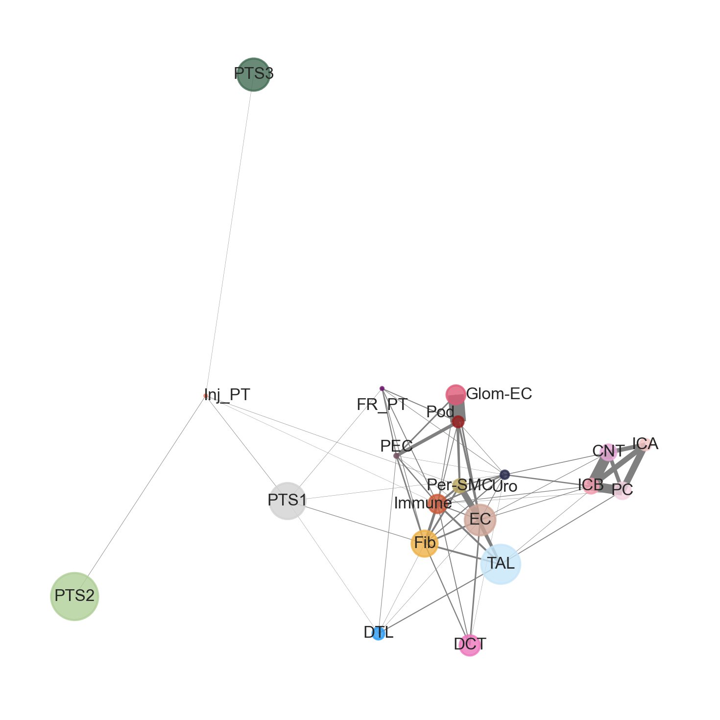
Within the Sham sample, two primary colocalization structures {Glom-EC, Pod, PEC} and {CNT, ICA, ICB, PC} can be seen. In contrast, there appears to be a weak colocalization between {PTS2, PTS3, and Inj_PT}
Section III: Xenium and Visium Dataset Alignment
In this study, the Xenium dataset contains a panel of 300 genes, but well defined cell segmentation (Baysor). The Visium dataset contains up to ~20,000 genes but coarse tissue resolution. Aligning the two forms of datasets (for the same or similar type of tissue) bridges the advantages of each platform and gives a more complete analysis.
From Xenium, we defined tissue subregions (CN 0, CN 1) corresponding to unique structural arrangements in kidneys. We can transfer these subregions onto the visium dataset, and perform DEG, TF, Pathway, and LR analyses, taking advantage of visium's high transcriptomic ~20,000 gene depth.
The authors performed Xenium and Visum Dataset alignment for all six samples. For the purpose of this demonstration, only the Sham sample will be analyzed.
def align(H, adata_xe, adata_vis):

    ### convert HE coordinates to Xenium DAPI coordinates and scale
    points_vis = np.array(adata_vis.obs[["X_coords","Y_coords"]])
    points_vis2 = np.hstack((points_vis, np.ones((points_vis.shape[0], 1))))
    points_xe = np.dot(points_vis2, H.T)
    points_xe2 = points_xe[:, :2] / points_xe[:, 2, np.newaxis]
    points_xe2 = points_xe2*0.2125

    fig, axs = plt.subplots(1,2,dpi=100)
    axs[0].scatter(points_xe2[:,0], points_xe2[:,1],  marker='o', linewidth=0, alpha=1, color="black", s=15)
    axs[0].axis('scaled')
    axs[1].scatter(adata_xe.obs["x_centroid"], adata_xe.obs["y_centroid"],  marker='o', linewidth=0, alpha=1, color="black", s=1)
    axs[1].axis('scaled')
    plt.show()

    return points_xe2
def register_xenium_visium(adata_xe, adata_vis, spot_diameter=100):

    from scipy.spatial.distance import cdist

    df_xenium = adata_xe.obs[['x_centroid', 'y_centroid','celltype_plot']]
    df_xenium["cell_id"] = df_xenium.index.tolist()

    df_visium =  adata_vis.obs[["x_align","y_align"]]
    df_visium["spot_id"] = df_visium.index.tolist()
    distances = cdist(df_xenium[['x_centroid', 'y_centroid']], df_visium[["x_align","y_align"]], metric='euclidean')
    print(distances.shape)

    print("Visium x_align/y_align NA?:",
      adata_vis.obs[["x_align","y_align"]].isna().any().to_dict())

    print("Xenium centroid NA?:",
      adata_xe.obs[["x_centroid","y_centroid"]].isna().any().to_dict())

    print("Visium coord range:",
      adata_vis.obs["x_align"].min(), adata_vis.obs["x_align"].max(),
      adata_vis.obs["y_align"].min(), adata_vis.obs["y_align"].max())

    print("Xenium coord range:",
      adata_xe.obs["x_centroid"].min(), adata_xe.obs["x_centroid"].max(),
      adata_xe.obs["y_centroid"].min(), adata_xe.obs["y_centroid"].max())

    print("Min distance overall:", np.nanmin(distances))
    print("Fraction within radius:", np.mean(distances <= (spot_diameter/2)))

    include_cells = distances <= (spot_diameter / 2)
    print("Mapping Xenium cells to Visium spots.....")
    # Create a DataFrame for cell to spot correspondence
    corr_df = pd.DataFrame([{'cell_id': adata_xe.obs_names[cell_idx],
                             'spot_id': adata_vis.obs_names[spot_idx]}
                            for cell_idx, row in enumerate(include_cells)
                            for spot_idx, within in enumerate(row) if within])

    # Ensure the order of spots matches the Visium data
    #ordered_index = adata_vis.obs[adata_vis.obs.index.isin(corr_df.spot_id.tolist())].index
    ordered_index = adata_vis.obs.index[adata_vis.obs.index.isin(corr_df["spot_id"])]
    print(f"Original Xenium cell #: {adata_xe.shape[0]}, mapped Xenium cell #:{corr_df.shape[0]}")

    gene_overlap = [g for g in adata_xe.var_names if g in adata_vis.var_names]
    # Aggregate gene expression for cells within each spot
    print("Calculating psudobulk Xenium data.....")
    count_df = sc.get.obs_df(adata_xe, keys=gene_overlap, use_raw=True)
    agg_gene = []

    for spot_id in adata_vis.obs_names:
        cells_in_spot = corr_df[corr_df['spot_id'] == spot_id]['cell_id']
        counts = count_df.loc[cells_in_spot.tolist(),]
        sum_counts = counts.sum(axis=0).to_numpy()
        agg_gene.append(sum_counts)

    agg_gene_df = pd.DataFrame(agg_gene, columns=gene_overlap, index=adata_vis.obs_names)
    agg_gene_df.fillna(0, inplace=True)

    ## check the aggregation by aggregating genes and calculate correlation
    agg_gene_df = agg_gene_df.loc[adata_vis.obs.index,]
    Xenium_agg_gene_df = agg_gene_df.loc[:,gene_overlap]
    Visium_gene_df = sc.get.obs_df(adata_vis, keys = gene_overlap, use_raw=True)

    corr = pd.DataFrame(Xenium_agg_gene_df.corrwith(Visium_gene_df, method = "pearson",), columns = ["pearson_r"])
    corr[corr["pearson_r"]<=0] = 0
    corr = corr.fillna(0)
    print("Top 5 correlated spatial gene expression .....")
    print(corr.sort_values(by = "pearson_r", ascending=False).head(10))

    return corr_df, Xenium_agg_gene_df
xe_adata = sc.read_h5ad("Xenium_all.h5ad")
adata_vis = sc.read_h5ad("visium_fullres_all.h5ad")
adata_vis = adata_vis[adata_vis.obs["ident"].isin(['ShamR','Hour4R','Hour12R', 'Day2R', 'Day14R', 'Week6R'])]
sham_vis = adata_vis[adata_vis.obs.ident == "ShamR"]
x = sham_vis.obs["X_coords"]
y = sham_vis.obs["Y_coords"]
fig, ax = plt.subplots(dpi=100)
ax.scatter(x, y,  marker='o', linewidth=0, alpha=1, color="black", s=15)
ax.axis('scaled')
ax.invert_yaxis()
plt.show()
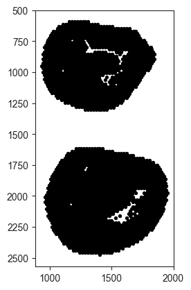
Cropping Images for analysis
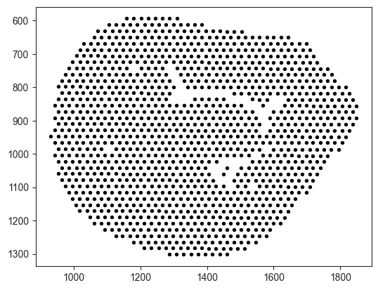
The above image contains two tissue slides, but we only need the one below y = 1500 to run alignment. We can use the following code to partition the slides according to their x and y coordinates.
mask = sham_vis.obs["Y_coords"] < 1500

sham_vis = sham_vis[mask].copy()

x = sham_vis.obs["X_coords"]
y = sham_vis.obs["Y_coords"]

fig, ax = plt.subplots(dpi=100)
ax.scatter(x, y,  marker='o', linewidth=0, alpha=1, color="black", s=15)
ax.axis('scaled')
ax.invert_yaxis()
plt.show()
Realign Spatial Samples
Ensure that Visium tissue (left) is on the same scale and orientation as the Xenium tissue (right). The spatial transformation vector was provided by the authors.
H = np.array([[0.09405798593520641,-3.41158653187994,-959.2731416178372],
             [-3.41158653187994,-0.09405798593520641,-1528.8859782583281],
             [0,0,1]])

sham_xe = xe_adata[xe_adata.obs.ident=="ShamR"]
points_xe2 = align(H, sham_xe, sham_vis)
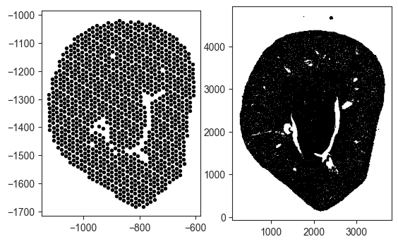
Rescaling Coordinates for Alignment
Note that the coordinates are also mismatched (Visium coordinates are negative while Xenium coordinates are positve). Rescaling the Visium coordinates to the min, max of the respective Xenium coordinates is necessary.
# Xenium target ranges
xe_x_min, xe_x_max = sham_xe.obs["x_centroid"].min(), sham_xe.obs["x_centroid"].max()
xe_y_min, xe_y_max = sham_xe.obs["y_centroid"].min(), sham_xe.obs["y_centroid"].max()

# Current Visium-aligned ranges
vis_x_min, vis_x_max = points_xe2[:,0].min(), points_xe2[:,0].max()
vis_y_min, vis_y_max = points_xe2[:,1].min(), points_xe2[:,1].max()

# Rescale X
x_scaled = (points_xe2[:,0] - vis_x_min) / (vis_x_max - vis_x_min)
x_scaled = x_scaled * (xe_x_max - xe_x_min) + xe_x_min

# Rescale Y
y_scaled = (points_xe2[:,1] - vis_y_min) / (vis_y_max - vis_y_min)
y_scaled = y_scaled * (xe_y_max - xe_y_min) + xe_y_min

points_xe2 = np.column_stack([x_scaled, y_scaled])
sham_vis.obs[["x_align","y_align"]] = points_xe2
sham_corr_df, sham_Xenium_agg_gene_df = register_xenium_visium(sham_xe, sham_vis, spot_diameter=55)
(85880, 1224)
Visium x_align/y_align NA?: {'x_align': False, 'y_align': False}
Xenium centroid NA?: {'x_centroid': False, 'y_centroid': False}
Visium coord range: 263.8611838888889 3652.423685416667 153.7642375 4704.941791875
Xenium coord range: 263.8611838888889 3652.423685416667 153.7642375 4704.941791875
Min distance overall: 0.12524308632228534
Fraction within radius: 0.00019696125616835774
Mapping Xenium cells to Visium spots.....
Original Xenium cell #: 85880, mapped Xenium cell #:20704
Calculating psudobulk Xenium data.....
Top 5 correlated spatial gene expression .....
          pearson_r
Slc12a1    0.568569
Epcam      0.537867
Ptger3     0.535578
Cyp7b1     0.532829
Plau       0.524735
Slc5a3     0.508235
Umod       0.484839
Slc22a19   0.466614
Cd24a      0.462949
Aqp1       0.462512
# save correlation map
sham_corr_df.to_csv("Xe2vis_sham_map_df_diameter_55um.csv")
A mapping table will allow you to link metadata variables from the xenium data (rownames being cell_id) onto the visium data (rownames being spot_id).
sham_corr_df
| cell_id | spot_id | |
|---|---|---|
| 0 | ShamR_1 | ShamR_GCGTACCGCAAGCGAA-1 |
| 1 | ShamR_3 | ShamR_GCGTACCGCAAGCGAA-1 |
| 2 | ShamR_5 | ShamR_GCGTACCGCAAGCGAA-1 |
| 3 | ShamR_6 | ShamR_GCGTACCGCAAGCGAA-1 |
| 4 | ShamR_8 | ShamR_GCGTACCGCAAGCGAA-1 |
| ... | ... | ... |
| 20699 | ShamR_94464 | ShamR_GTTGTCCTTGCTTAGC-1 |
| 20700 | ShamR_94468 | ShamR_GTTGCTGTCTGTAACT-1 |
| 20701 | ShamR_94560 | ShamR_TGGTTGGATTAATGAT-1 |
| 20702 | ShamR_94630 | ShamR_CTCATATGCACCGTCT-1 |
| 20703 | ShamR_94710 | ShamR_CGGTGAGCGTTGAGCG-1 |
20704 rows × 2 columns
You can append the celltype_plot, region, and CN onto the Visium data, and run cell-cell communication, differential gene expression, and functional enrichment on the updated Visium data.
# Pull desired metadata from Xenium
xe_meta = sham_xe.obs[["celltype_plot", "region", "CN"]].copy()
xe_meta["cell_id"] = xe_meta.index

# Merge into mapping table
corr_annot = sham_corr_df.merge(xe_meta, on="cell_id", how="left")
def majority_vote(series):
    return series.value_counts().idxmax()

spot_majority = (
    corr_annot
    .groupby("spot_id")[["celltype_plot", "region", "CN"]]
    .agg(majority_vote)
)
sham_vis.obs = sham_vis.obs.join(spot_majority)
sham_vis.obs['CN'].value_counts()
CN
CN2: Cortical Proximal Tubule     499
CN0: Loop of Henle                200
CN3: Medullary Proximal Tubule    159
CN6: Distal Tubule Niche           83
CN5: Collecting Duct Niche         76
CN1: Glomerular Niche              47
CN8: Uro-immune Niche               8
CN7: Fibro-inflammatory Niche       3
CN4: Injured Proximal Tubule        0
Name: count, dtype: int64
Section IV: Differential Expression and Cell-Cell Interaction
To identify genes that distinguish specific spatial niches or cell populations, the authors performed differential gene expression analysis using the Visium whole-transcriptome data. After transferring Xenium-defined neighborhood labels (e.g., fibro-inflammatory niche CN7) onto Visium spots, they compared gene expression between spots belonging to a given niche and all other spots.
Statistical testing (using standard single-cell tools such as Scanpy functions) identified genes that were significantly upregulated within each niche. This approach allowed them to define molecular signatures characteristic of injured tubule regions or fibrotic microenvironments, which will be used for downstream pathway and transcription factor analyses.
# Create binary group (CN3 vs Other)
sham_vis.obs['CN_binary'] = np.where(
    sham_vis.obs['CN'].str.contains('CN3', na=False),
    'CN3',
    'Other'
)

print(sham_vis.obs['CN_binary'].value_counts())
CN_binary
Other    1065
CN3       159
Name: count, dtype: int64
use_raw = True if sham_vis.raw is not None else False

sc.tl.rank_genes_groups(
    sham_vis,
    groupby='CN_binary',
    groups=['CN3'],
    reference='Other',
    method='wilcoxon',
    pts=True,            # include percent expressed columns
    key_added='rank_CN3_vs_Other'
)

# convert to dataframe
deg_df = sc.get.rank_genes_groups_df(sham_vis, group='CN3', key='rank_CN3_vs_Other')
deg_df.head()
| names | scores | logfoldchanges | pvals | pvals_adj | pct_nz_group | |
|---|---|---|---|---|---|---|
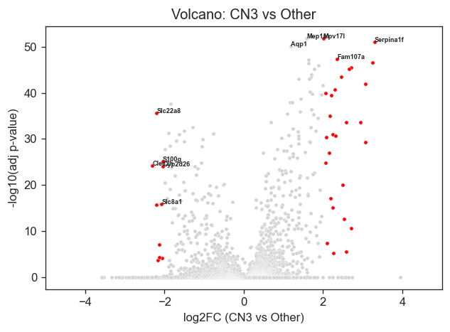
| 0 | Mep1a | 15.884229 | 1.582605 | 8.149371e-57 | 1.450075e-52 | 1.000000 |
| 1 | Mpv17l | 15.846348 | 2.002293 | 1.489930e-56 | 1.450075e-52 | 1.000000 |
| 2 | Serpina1f | 15.710214 | 3.301317 | 1.287445e-55 | 8.353375e-52 | 0.930818 |
| 3 | Aqp1 | 15.543173 | 1.191752 | 1.769978e-54 | 8.613157e-51 | 1.000000 |
| 4 | Fam107a | 15.125272 | 2.349711 | 1.103443e-51 | 4.295704e-48 | 0.968553 |
# Add BH-adjusted p-value (Scanpy returns pvals_adj sometimes already named)
if 'pvals_adj' not in deg_df.columns and 'pvals' in deg_df.columns:
    deg_df['pvals_adj'] = sc.tl._utils._fdr_bh(deg_df['pvals'])  # internal helper might not exist everywhere

sig = deg_df[(deg_df['pvals_adj'] < 0.05) & (abs(deg_df['logfoldchanges']) > 2)].copy()
print(f"Significant genes: {sig.shape[0]}")
sig.head(50)
Significant genes: 38
| names | scores | logfoldchanges | pvals | pvals_adj | pct_nz_group | neglog10_p | score | |
|---|---|---|---|---|---|---|---|---|
| 1 | Mpv17l | 15.846348 | 2.002293 | 1.489930e-56 | 1.450075e-52 | 1.000000 | 51.838610 | 111.781672 |
| 2 | Serpina1f | 15.710214 | 3.301317 | 1.287445e-55 | 8.353375e-52 | 0.930818 | 51.078138 | 181.210171 |
| 4 | Fam107a | 15.125272 | 2.349711 | 1.103443e-51 | 4.295704e-48 | 0.968553 | 47.366966 | 119.734808 |
| 6 | Cyp7b1 | 14.971219 | 3.252325 | 1.132261e-50 | 3.148496e-47 | 0.905660 | 46.501897 | 162.440789 |
| 9 | Mep1b | 14.779406 | 2.703557 | 1.989142e-49 | 3.871865e-46 | 0.930818 | 45.412080 | 131.666822 |
| 10 | Slc22a13 | 14.724327 | 2.662522 | 4.499287e-49 | 7.920397e-46 | 0.930818 | 45.101253 | 128.724561 |
| 13 | Cryab | 14.462041 | 2.449461 | 2.104637e-47 | 2.926198e-44 | 0.993711 | 43.533696 | 114.333034 |
| 17 | Serpina1d | 14.194102 | 3.070361 | 9.965376e-46 | 1.077645e-42 | 0.867925 | 41.967524 | 138.170876 |
| 19 | Irx1 | 13.979320 | 2.288296 | 2.084722e-44 | 2.028956e-41 | 0.974843 | 40.692727 | 99.954957 |
| 21 | Gpm6a | 13.844870 | 2.072563 | 1.366290e-43 | 1.208856e-40 | 0.955975 | 39.917625 | 88.839295 |
| 24 | Ppic | 13.770068 | 2.200595 | 3.858502e-43 | 3.004230e-40 | 0.924528 | 39.522267 | 93.335111 |
| 32 | Napsa | 12.980926 | 2.173947 | 1.569724e-38 | 8.729910e-36 | 0.899371 | 35.058990 | 82.184289 |
| 34 | Scd1 | 12.730545 | 2.574710 | 4.000359e-37 | 2.104513e-34 | 0.823899 | 33.676848 | 93.714027 |
| 36 | Slc22a19 | 12.713709 | 2.946467 | 4.962380e-37 | 2.476737e-34 | 0.779874 | 33.606120 | 106.969440 |
| 41 | Hsd11b1 | 12.223772 | 2.244354 | 2.320622e-34 | 9.218554e-32 | 0.855346 | 31.035337 | 75.487506 |
| 43 | Rnf24 | 12.158591 | 2.306032 | 5.164153e-34 | 1.970985e-31 | 0.842767 | 30.705317 | 76.760887 |
| 45 | Agt | 12.091607 | 2.077393 | 1.169764e-33 | 4.296122e-31 | 0.861635 | 30.366923 | 68.412512 |
| 50 | Bcat1 | 11.876703 | 3.071159 | 1.564156e-32 | 4.991196e-30 | 0.723270 | 29.301795 | 97.680427 |
| 57 | Myo5a | 11.398912 | 2.160543 | 4.233754e-30 | 1.160704e-27 | 0.792453 | 26.935278 | 63.462214 |
| 64 | Slc38a3 | 10.958402 | 2.072758 | 6.055927e-28 | 1.473483e-25 | 0.786164 | 24.831655 | 56.415958 |
| 83 | Higd1c | 9.876307 | 2.485729 | 5.274065e-23 | 9.332697e-21 | 0.641509 | 20.029993 | 55.376719 |
| 101 | Slco4c1 | 9.134307 | 2.183498 | 6.582726e-20 | 9.218184e-18 | 0.622642 | 17.035355 | 41.882966 |
| 114 | Apoa4 | 8.619717 | 2.236037 | 6.712013e-18 | 8.064774e-16 | 0.597484 | 15.093408 | 38.399785 |
| 134 | Sec14l3 | 7.924617 | 2.527192 | 2.288510e-15 | 2.249790e-13 | 0.503145 | 12.647858 | 36.999219 |
| 157 | Akr1c18 | 7.277501 | 2.707819 | 3.400613e-13 | 2.865495e-11 | 0.446541 | 10.542800 | 33.762286 |
| 200 | A4gnt | 6.197932 | 2.108439 | 5.721000e-10 | 3.736888e-08 | 0.427673 | 7.427490 | 19.487311 |
| 234 | Itih2 | 5.413960 | 2.584618 | 6.164587e-08 | 3.351779e-06 | 0.333333 | 5.474725 | 18.635345 |
| 246 | Ceacam2 | 5.295505 | 2.267661 | 1.186882e-07 | 6.160707e-06 | 0.345912 | 5.210369 | 15.704895 |
| 19282 | Ces1g | -4.525243 | -2.164013 | 6.032618e-06 | 2.416151e-04 | 0.088050 | 3.616876 | -11.295053 |
| 19311 | Pvalb | -4.801599 | -2.054794 | 1.574036e-06 | 7.039877e-05 | 0.132075 | 4.152435 | -11.923941 |
| 19315 | Gldc | -4.832145 | -2.120764 | 1.350698e-06 | 6.117961e-05 | 0.100629 | 4.213393 | -12.447701 |
| 19360 | Npl | -6.067330 | -2.137418 | 1.300543e-09 | 8.166152e-08 | 0.119497 | 7.087983 | -18.992830 |
| 19418 | Slc5a12 | -8.768598 | -2.201866 | 1.809053e-18 | 2.257258e-16 | 0.245283 | 15.646419 | -39.066709 |
| 19419 | Slc8a1 | -8.810568 | -2.070154 | 1.245132e-18 | 1.584084e-16 | 0.433962 | 15.800222 | -37.065665 |
| 19447 | Cyp2d26 | -10.774526 | -2.036326 | 4.541187e-27 | 1.064990e-24 | 0.415094 | 23.972654 | -53.642602 |
| 19449 | Clec2h | -10.835857 | -2.304983 | 2.327741e-27 | 5.593762e-25 | 0.327044 | 24.252296 | -61.388773 |
| 19451 | S100g | -11.017570 | -2.048655 | 3.144343e-28 | 7.846749e-26 | 0.899371 | 25.105310 | -56.343080 |
| 19463 | Slc22a8 | -13.088077 | -2.198809 | 3.852401e-39 | 2.343343e-36 | 0.635220 | 35.630164 | -84.465645 |
Volcano plot(s) of the top differentially expressed genes (CN3 vs other regions) can be generated through the following.
genes_to_label = ["Mep1a", "Mpv17l", "Serpina1f", "Aqp1", "Fam107a", "Slc22a8", "S100g", "Clec2h", "Cyp2d26", "Slc8a1"]

# Compute y values once
deg_df["neglog10_p"] = -np.log10(deg_df["pvals_adj"] + 1e-300)

plt.figure(figsize=(6,4), dpi=120)

# All genes
sns.scatterplot(
    x=deg_df["logfoldchanges"],
    y=deg_df["neglog10_p"],
    s=10,
    color="lightgray"
)

# Significant genes
sns.scatterplot(
    x=sig["logfoldchanges"],
    y=-np.log10(sig["pvals_adj"] + 1e-300),
    color="red",
    s=10
)

# ---- Label chosen genes ----
label_df = deg_df[deg_df["names"].isin(genes_to_label)]

for _, row in label_df.iterrows():
    plt.text(
        row["logfoldchanges"],
        row["neglog10_p"],
        row["names"],
        fontsize=5.5,
        fontweight="bold"
    )

plt.xlabel("log2FC (CN3 vs Other)")
plt.ylabel("-log10(adj p-value)")
plt.title("Volcano: CN3 vs Other")
plt.xlim(-5,5)
plt.show()
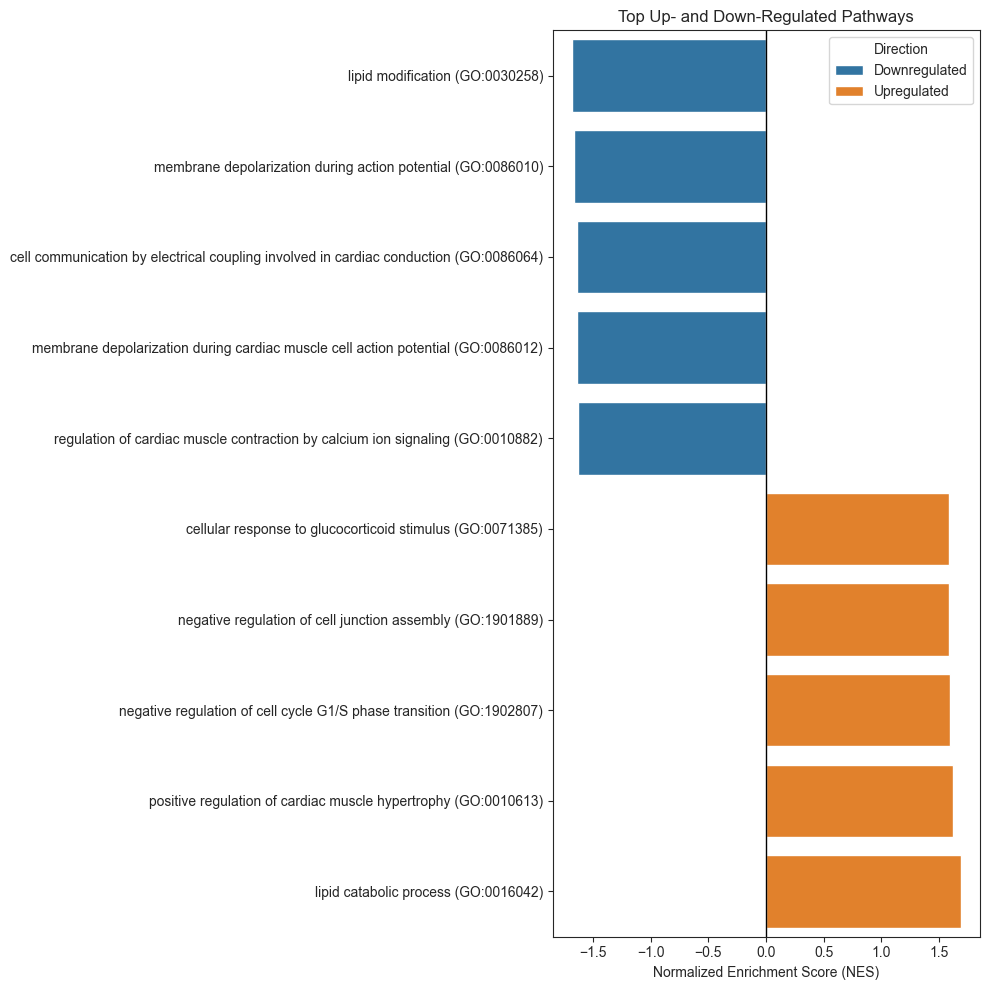
Functional Enrichment (Biological Pathway) Analysis
Pathway and gene ontology enrichment analysis to determine the biological processes represented by those gene sets. Curated gene collections such as MSigDB Hallmark pathways and Gene Ontology Biological Process terms were used, accessed via tools like Enrichr.
By testing whether niche-specific gene lists were overrepresented in known biological pathways, they could infer functional programs active in each region.
# Build a preranked list: gene -> score (here use signed score: logFC * -log10(pval))
deg_df['score'] = deg_df['logfoldchanges'] * -np.log10(deg_df['pvals'] + 1e-300)
rnk = deg_df[['names','score']].sort_values('score', ascending=False)

# run prerank GSEA
pre_res = gp.prerank(rnk=rnk, gene_sets='GO_Biological_Process_2021', organism='Mouse',
                     outdir=None, permutation_num=100)

# show top enriched sets
pre_res.res2d.head()
2026-05-18 15:16:10,760 [WARNING] Duplicated values found in preranked stats: 0.87% of genes
The order of those genes will be arbitrary, which may produce unexpected results.
| Name | Term | ES | NES | NOM p-val | FDR q-val | FWER p-val | Tag % | Gene % | Lead_genes | |
|---|---|---|---|---|---|---|---|---|---|---|
| 0 | prerank | lipid catabolic process (GO:0016042) | 0.956405 | 1.686283 | 0.023256 | 0.082013 | 0.07 | 5/20 | 2.20% | Hsd11b1;Apoa4;Acadl;Plaat3;Lpl |
| 1 | prerank | lipid modification (GO:0030258) | -0.907493 | -1.681775 | 0.0 | 1.0 | 0.69 | 1/37 | 0.04% | Cyp2e1 |
| 2 | prerank | membrane depolarization during action potentia... | -0.933388 | -1.664409 | 0.014706 | 1.0 | 0.85 | 1/26 | 0.11% | Slc8a1 |
| 3 | prerank | cell communication by electrical coupling invo... | -0.93445 | -1.642389 | 0.016949 | 1.0 | 0.98 | 1/16 | 0.11% | Slc8a1 |
| 4 | prerank | membrane depolarization during cardiac muscle ... | -0.962052 | -1.636651 | 0.0 | 1.0 | 0.99 | 1/17 | 0.11% | Slc8a1 |
res = pre_res.res2d.copy()

# Select top positive and negative pathways
top_up = res.sort_values("NES", ascending=False).head(5)
top_down = res.sort_values("NES", ascending=True).head(5)

plot_df = pd.concat([top_up, top_down])

# Color by direction
plot_df["Direction"] = np.where(plot_df["NES"] > 0,
                                "Upregulated",
                                "Downregulated")

# Sort for plotting
plot_df = plot_df.sort_values("NES")

plt.figure(figsize=(10, 10))

sns.barplot(
    data=plot_df,
    x="NES",
    y="Term",
    hue="Direction",
)

plt.axvline(0, color="black", lw=1)

plt.xlabel("Normalized Enrichment Score (NES)")
plt.ylabel("")
plt.title("Top Up- and Down-Regulated Pathways")

plt.tight_layout()
plt.show()
Ligand - Receptor (Cell-Cell) Communication through COMMOT
Neighboring cells were identified based on a defined radius. Then, using curated ligand–receptor databases (such as CellChat) and COMMOT (https://github.com/zcang/COMMOT), they assessed whether ligand genes expressed in one cell type corresponded to receptor genes expressed in adjacent cell types.
By focusing only on physically neighboring cells, the authors reduced false-positive signaling predictions common in non-spatial single-cell data. This analysis revealed strong signaling interactions—such as PDGF, TGF-β, chemokine, and integrin pathways—between failed-repair proximal tubule cells, fibroblasts, and immune cells, which may mediate the observed fibrosis progression.
adata_sub = sham_vis[sham_vis.obs["Y_coords"] < 1500].copy()
A) Expression matrix
COMMOT expects non-negative “abundance-like” values (typical: normalized counts + log1p).
sc.pp.normalize_total(adata_sub, inplace=True)
sc.pp.log1p(adata_sub)
WARNING: adata.X seems to be already log-transformed.
sc.pp.normalize_total(adata_sub); sc.pp.log1p(adata_sub)

# Note that Commot requires manual alignment of Xenium-Visium data
adata_sub.obsm["spatial"] = adata_sub.obs[["x_align","y_align"]].to_numpy()

# Load CellChat DB
df = ct.pp.ligand_receptor_database(database="CellChat", species="mouse", signaling_type=None)
df.columns = ["Ligand","Receptor","Pathway","Category"]

# Filter to PDGF pathway OR anything with ITGB2 in ligand/receptor (including heteromers like Itgal_Itgb2)
pdgf_df = df[df["Pathway"].str.contains("PDGF", case=False, na=False)]

itgb2_df = df[
    df["Ligand"].str.contains("Itgb2", case=False, na=False) |
    df["Receptor"].str.contains("Itgb2", case=False, na=False)
]

df_focus = pd.concat([pdgf_df, itgb2_df], ignore_index=True).drop_duplicates()

# Keep only pairs that exist in this dataset (and expressed in >=1% cells)
df_focus = ct.pp.filter_lr_database(df_focus, adata_sub, min_cell_pct=0.01)
# 4) Run commot spatial communication
ct.tl.spatial_communication(
    adata_sub,
    database_name="cellchat",
    df_ligrec=df_focus,
    dis_thr=100,
    heteromeric=True,
    pathway_sum=True
)

# 5) drop total columns if you don't want them
for key, dropcol in [
    ("commot-cellchat-sum-sender",   "s-total-total"),
    ("commot-cellchat-sum-receiver", "r-total-total"),
]:
    if key in adata_sub.obsm and dropcol in adata_sub.obsm[key].columns:
        adata_sub.obsm[key] = adata_sub.obsm[key].drop(columns=[dropcol])
adata_sub.obsm
AxisArrays with keys: X_pca, X_pca_harmony, X_umap, spatial, commot-cellchat-sum-sender, commot-cellchat-sum-receiver, commot_sender_vf-cellchat-Pdgfd-Pdgfrb, commot_receiver_vf-cellchat-Pdgfd-Pdgfrb
adata_sub.obsm['commot-cellchat-sum-sender']
| s-Icam2-Itgal_Itgb2 | s-Icam2-Itgam_Itgb2 | s-Itgal_Itgb2-Icam2 | s-Itgal_Itgb2-Cd226 | s-Itgal_Itgb2-Icam1 | s-Pdgfd-Pdgfrb | s-C3-Itgam_Itgb2 | s-F11r-Itgal_Itgb2 | s-Jam3-Itgam_Itgb2 | s-Thy1-Itgam_Itgb2 | ... | s-Pdgfb-Pdgfrb | s-Pdgfb-Pdgfra | s-CD40 | s-COMPLEMENT | s-GP1BA | s-ICAM | s-ITGAL-ITGB2 | s-JAM | s-PDGF | s-THY1 | |
|---|---|---|---|---|---|---|---|---|---|---|---|---|---|---|---|---|---|---|---|---|---|
| ShamR_AACAGGATGCTGGCAT-1 | 0.0 | 0.0 | 0.0 | 0.0 | 0.0 | 0.000000 | 0.0 | 0.0 | 0.0 | 0.0 | ... | 0.000000 | 0.000000 | 0.0 | 0.0 | 0.0 | 0.0 | 0.0 | 0.0 | 0.000000 | 0.0 |
| ShamR_AACATACTAGCCGAAG-1 | 0.0 | 0.0 | 0.0 | 0.0 | 0.0 | 0.367274 | 0.0 | 0.0 | 0.0 | 0.0 | ... | 0.000000 | 0.000000 | 0.0 | 0.0 | 0.0 | 0.0 | 0.0 | 0.0 | 0.367274 | 0.0 |
| ShamR_AACATATGCACTTCTA-1 | 0.0 | 0.0 | 0.0 | 0.0 | 0.0 | 0.000000 | 0.0 | 0.0 | 0.0 | 0.0 | ... | 0.000000 | 0.000000 | 0.0 | 0.0 | 0.0 | 0.0 | 0.0 | 0.0 | 0.000000 | 0.0 |
| ShamR_AACATCAACATCTTGA-1 | 0.0 | 0.0 | 0.0 | 0.0 | 0.0 | 0.000000 | 0.0 | 0.0 | 0.0 | 0.0 | ... | 0.000000 | 0.000000 | 0.0 | 0.0 | 0.0 | 0.0 | 0.0 | 0.0 | 0.000000 | 0.0 |
| ShamR_AACATGCACTTCGGAT-1 | 0.0 | 0.0 | 0.0 | 0.0 | 0.0 | 0.000000 | 0.0 | 0.0 | 0.0 | 0.0 | ... | 0.000000 | 0.365302 | 0.0 | 0.0 | 0.0 | 0.0 | 0.0 | 0.0 | 0.365302 | 0.0 |
| ... | ... | ... | ... | ... | ... | ... | ... | ... | ... | ... | ... | ... | ... | ... | ... | ... | ... | ... | ... | ... | ... |
| ShamR_TGTTCACTTCACATAA-1 | 0.0 | 0.0 | 0.0 | 0.0 | 0.0 | 0.000000 | 0.0 | 0.0 | 0.0 | 0.0 | ... | 0.000000 | 0.000000 | 0.0 | 0.0 | 0.0 | 0.0 | 0.0 | 0.0 | 0.000000 | 0.0 |
| ShamR_TGTTCGATGGATACGT-1 | 0.0 | 0.0 | 0.0 | 0.0 | 0.0 | 0.000000 | 0.0 | 0.0 | 0.0 | 0.0 | ... | 0.000000 | 0.000000 | 0.0 | 0.0 | 0.0 | 0.0 | 0.0 | 0.0 | 0.000000 | 0.0 |
| ShamR_TGTTGGCCTGTAGCGG-1 | 0.0 | 0.0 | 0.0 | 0.0 | 0.0 | 0.000000 | 0.0 | 0.0 | 0.0 | 0.0 | ... | 0.000000 | 0.000000 | 0.0 | 0.0 | 0.0 | 0.0 | 0.0 | 0.0 | 0.000000 | 0.0 |
| ShamR_TGTTGGTGCGCACGAG-1 | 0.0 | 0.0 | 0.0 | 0.0 | 0.0 | 0.000000 | 0.0 | 0.0 | 0.0 | 0.0 | ... | 0.362103 | 0.000000 | 0.0 | 0.0 | 0.0 | 0.0 | 0.0 | 0.0 | 0.724206 | 0.0 |
| ShamR_TGTTGGTGCGCTTCGC-1 | 0.0 | 0.0 | 0.0 | 0.0 | 0.0 | 0.000000 | 0.0 | 0.0 | 0.0 | 0.0 | ... | 0.000000 | 0.000000 | 0.0 | 0.0 | 0.0 | 0.0 | 0.0 | 0.0 | 0.000000 | 0.0 |
1224 rows × 27 columns
pts = adata_sub.obsm['spatial']
s = adata_sub.obsm['commot-cellchat-sum-sender']['s-PDGF']
r = adata_sub.obsm['commot-cellchat-sum-sender']['s-ICAM']
fig, ax = plt.subplots(1,2, figsize=(10,8))
ax[0].scatter(pts[:,0], pts[:,1], c=s, s=40, cmap='bwr', marker = 'h')
ax[0].set_title('Sender - PDGF Signaling')
ax[1].scatter(pts[:,0], pts[:,1], c=r, s=40, cmap='bwr', marker = 'h')
ax[1].set_title('Sender - ICAM Signaling')
Text(0.5, 1.0, 'Sender - ICAM Signaling')
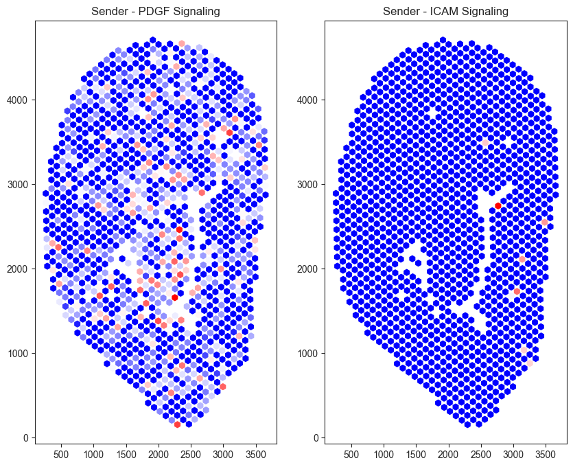
Sham tissue exhibits elevated PDGF (Platelet-Derived Growth Factor) signaling and comparatively low ICAM (Intercellular Adhesion Molecule) signaling. One possible explanation is that, immediately following injury, platelet- and stromal-associated signaling promotes vascular stabilization and early tissue remodeling. At this stage, inflammation and immune cell recruitment has likely not occurred, resulting in relatively low ICAM-mediated signaling.
Summary and Notes
This workflow demonstrates how multimodal spatial transcriptomics can be used to characterize the molecular and spatial dynamics of kidney injury and repair.
Through clustering, differential expression, and spatial permutation testing, distinct cellular niches associated with injury and fibrosis were identified. A notable example was how injured proximal tubule cells (Inj_PT) and PTS2 cells proportions changed over the course of repair. Spatially resolved signaling pathways, including PDGF and ICAM-associated interactions, further illustrate how communication between neighboring cells may contribute to chronic tissue remodeling following acute kidney injury.
By integrating Xenium and Visium datasets, the analysis combines the strengths of high-resolution cellular segmentation with whole-transcriptome profiling, enabling comprehensive investigation of tissue architecture, cell-state transitions, and spatial signaling networks.
To reduce computation time and simplify visualizations, subclassifications of Inj-PT cells were not used. The Sham tissue sample was used for Differential Expression, Pathway Enrichment, Network Analysis, and Cell-Cell Interaction.