Lesson 3: Creating a feature table

Lesson Objectives

• Check for primers
• Generate an ASV count table and representative sequence file
• Understand the difference between OTU picking and denoising

The two primary files that will be used throughout any microbiome analysis are the

1. feature table (OTU / ASV count data)
2. feature data (representative sequences).

These will be generated using either an OTU clustering method or a denoising method. The goal is to end up with counts of features, whether these be OTUs or ASVs (ESVs, zOTUs, etc.). Ideally, these features represent an organism or species of organisms.

But first...

Depending on your library preparation protocol, you may or may not have primers in your sequences. Non-biological sequences (e.g., adapters, primers, linker pads, etc.) can pose problems for OTU clustering and denoising (e.g., by interfering with chimera identification).

Primers are generally not found in sequences when using the EMP protocol due to the use of custom sequencing primers, but most other library prep strategies will result in primers in the sequences.

We can use qiime cutadapt to trim primers. If you are unsure whether to expect primers or not, it's a good idea to use qiime cutadapt to check for the presence of primers.

Primer trimming

Using qiime cutadapt trim-paired

We will use qiime cutadapt trim-paired because we are working with paired-end reads. We will also use more than one thread (--p-cores). The region sequenced was V4-V5 with the forward primer, AYTGGGYDTAAAGNG, and the reverse primer, CCGTCAATTYHTTTRAGT, which will fill the --p-front-f and --p-front-r parameters respectively. We will also specify that we want the command to run in --verbose mode so that we can save the output from cutadapt to a log for our records.

qiime cutadapt trim-paired \
--i-demultiplexed-sequences demuxsequences.qza \
--p-cores 8 \
--p-front-f AYTGGGYDTAAAGNG \
--p-front-r CCGTCAATTYHTTTRAGT \
--verbose \
--o-trimmed-sequences demux-trimmed.qza | tee cutadaptresults.log

For the most part, it seems that the primers are not in the sequences, aside from a 4 bp match. I wouldn't worry about these 4 bp unless something seems off in later analyses. From the overall length of the sequences, ~220 bp forward and ~217 bp reverse, it seems that the primers have likely been trimmed.

OTU Clustering vs Denoising

Once we have removed non-biological sequences, we can proceed to OTU clustering or denoising.

What do we mean by OTU Clustering / OTU picking?

An OTU is an operational taxonomic unit. This is derived by binning sequences at a certain threshold of similarity. This threshold is generally set at 97%, which is associated with a species level assignment.

Clustering can

1. eliminate variation added by sequencing error

2. avoid splitting counts from one organism, as bacteria have more than one 16S rRNA gene (average 4 copies), which may differ.

3. give you an idea of "species" counts; though, there may be important phenotypic differences between strains of a species.

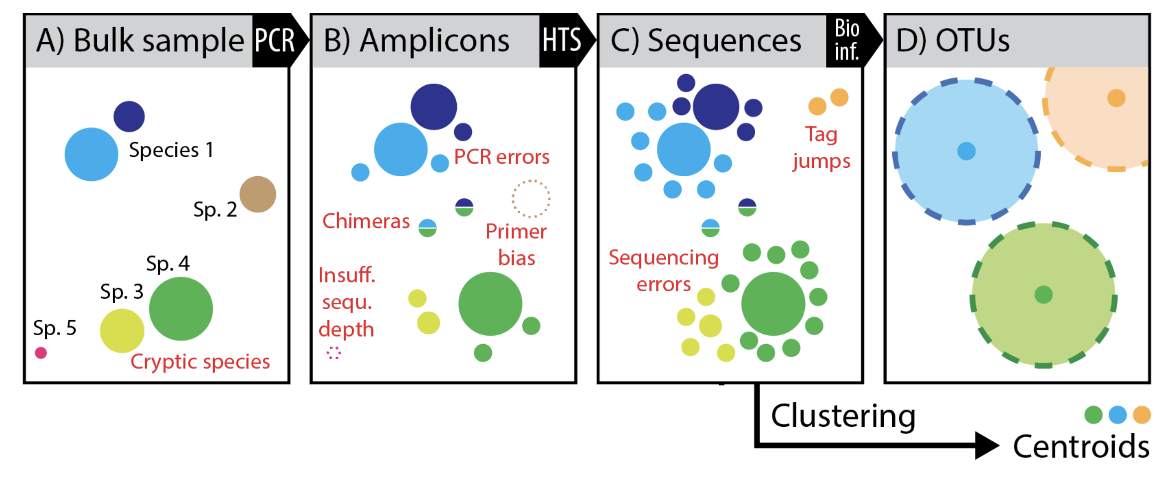
Figure modified slightly from Elbrecht V, Vamos EE, Steinke D, Leese F. 2018. Estimating intraspecific genetic diversity from community DNA metabarcoding data. PeerJ 6:e4644 https://doi.org/10.7717/peerj.4644 Supplemental Figure 1.

This image nicely outlines the biases and errors that accumulate from sample collection to sequencing and how those errors culminate in OTUs. First, with amplification you may have some primer bias, misrepresentation by sequencing depth, and chimera formation (B) then with high throughput sequencing we include sequencing error complicated by things like tag jumping in metabarcode studies. What we end up with if we cluster into OTUs is a cluster of sequences (represented usually by a single dominant sequence) considered to be a microbial species, but in reality this species could be multiple species and erroneous sequences clustered together. For example, the yellow and green species were lumped together. Also, only the representative sequence of the group will later be used for taxonomic classification and tree generation.

Methods for OTU clustering include

1. Closed reference OTU picking

   • uses a reference database to cluster OTUs against
   • reads that fail to cluster with a reference sequence due to real variation or sequence error variation are dropped
   • subject to biases or errors in databases; lose any newly recovered taxa
   • Can be used to compare studies if the same reference is used

2. De novo OTU picking

   • creates clusters of sequences based only on the observed sequences (no reference database)
   • Cannot be compared across studies

3. Open reference OTU picking (combination of 1 and 2)

   • a combination of closed-reference and de novo
   • sequences are clustered based on a reference
   • sequences that fail to cluster to a reference sequence are clustered using a de novo method
   • Cannot be compared across studies

Some potential reference databases include Greengenes, SILVA, and UNITE (for ITS fungi).

Clustering methods on QIIME 2

1. q2-dbotu
2. q2-vsearch

Denoising

The field has moved to denoising sequences rather than OTU clustering. In a denoising approach, the exact biological sequence is inferred and noise is removed from the dataset via error correction. This is generally done using some type of error modeling, dependent on sequence quality information. More details here.

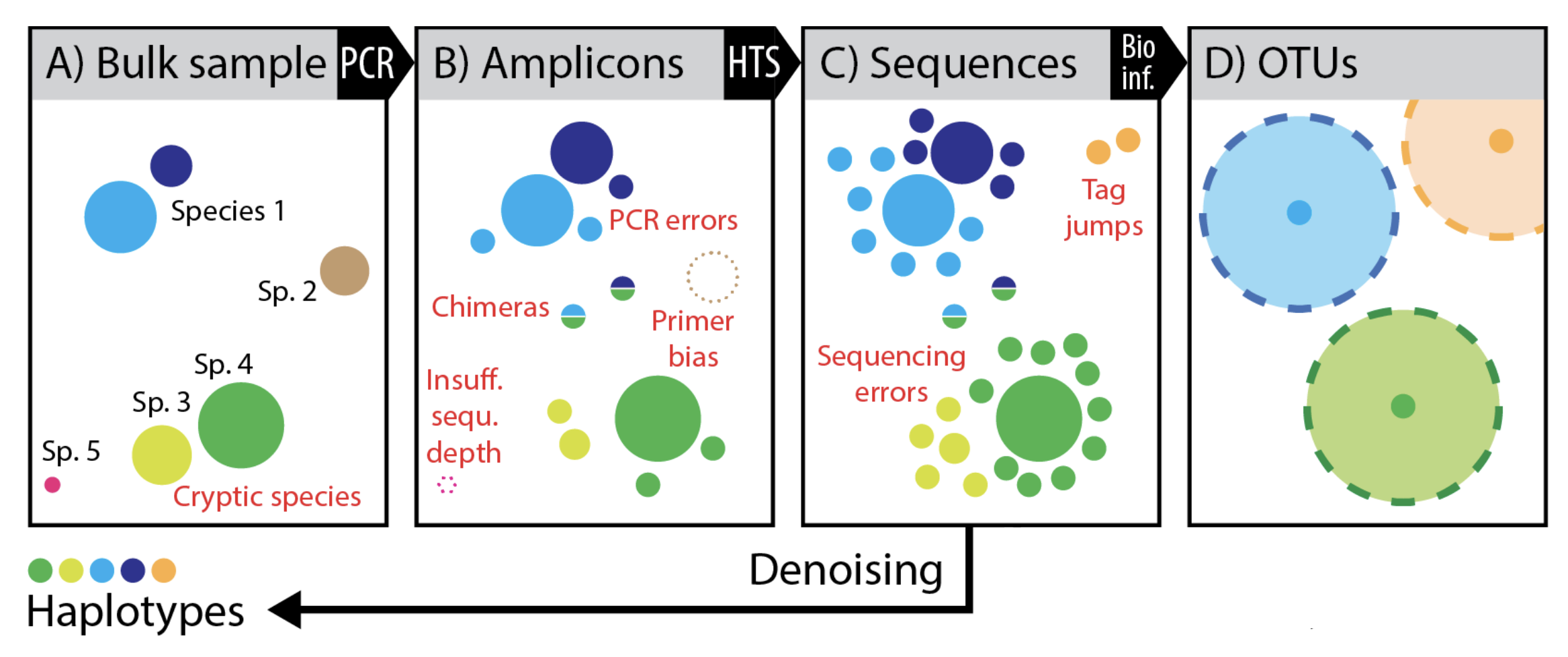
Figure modified slightly from Elbrecht V, Vamos EE, Steinke D, Leese F. 2018. Estimating intraspecific genetic diversity from community DNA metabarcoding data. PeerJ 6:e4644 https://doi.org/10.7717/peerj.4644 Supplemental Figure 1.

Back to our figure from Elbrecht et al. 2018, we can see that we get much greater resolution of the original diversity, when we remove sequences impacted by error. Though, we could have inflated diversity in the case of a single organism having multiple 16S rRNA copies with 1-2 nucleotide differences.

Denoising methods on QIIME2

The two methods used for denoising on QIIME 2 include:

DADA2
- Uses a run specific error profile
- Unclear how an incomplete run profile would impact results
- There is a method available for Pacbio CCS sequences

Deblur
- Not run specific, uses a fixed model
- Does not include an inherent read joining step (will drop reverse reads)
- Can read join before denoising

Related methods include:

Minimum Entropy Decomposition (MED)
Unoise3

Note: Each of these methods calls the resulting features something different (e.g., ASVs, zOTUs, sOTUs, etc.).

For a comparison of DADA2, Deblur, and Unoise3, see Denoising the Denoisers: an independent evaluation of microbiome sequence error-correction approaches.

For an interesting discussion on OTUs and ASVs, see this QIIME 2 forum post.

Also...You can do both denoising and OTUclustering! See qiime vsearch cluster-features-open-reference

Preparing to Denoise (Hands on)

Now that we know what we mean by denoising, let's apply it to our data. We will use DADA2, which seems to be the more popular method. To use DADA2, we need to make some decisions regarding the quality of our data. This means we need to refer back to our output from qiime demux summarize. In particular, we want to trim where the reads (forward and reverse) drop in quality. We can also trim any low quality bases from the beginning of the reads. However, we need to be wary of the length of our sequences (forward and reverse), the size of our target amplicon, and the general size of the overlap (between forward and reverse for merging). If we trim too much, we could impact our ability to merge the reads. Our primers are 563F and 926R, targeting V4-V5, so we are expecting a 363 bp amplicon. Because we are using 250 PE sequencing we can use the following to calculate approximate overlap:

(forward read) + (reverse read) - (length of amplicon) = overlap

250 + 250 - 363 = 137 bp overlap (Note: If primers were removed, it would not impact the overlap, so I'm going to ignore the current lengths in our summary report at the moment)

(See some explanations here and here.)

We need to trim based on quality but also recognize that sequences with lengths less than our truncation lengths will be removed, so we also need to consider our length table.

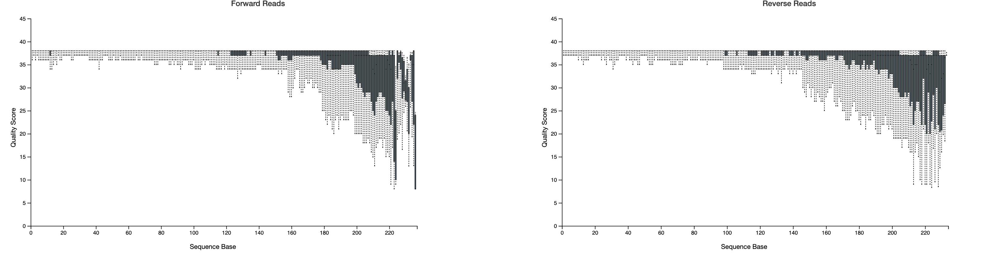
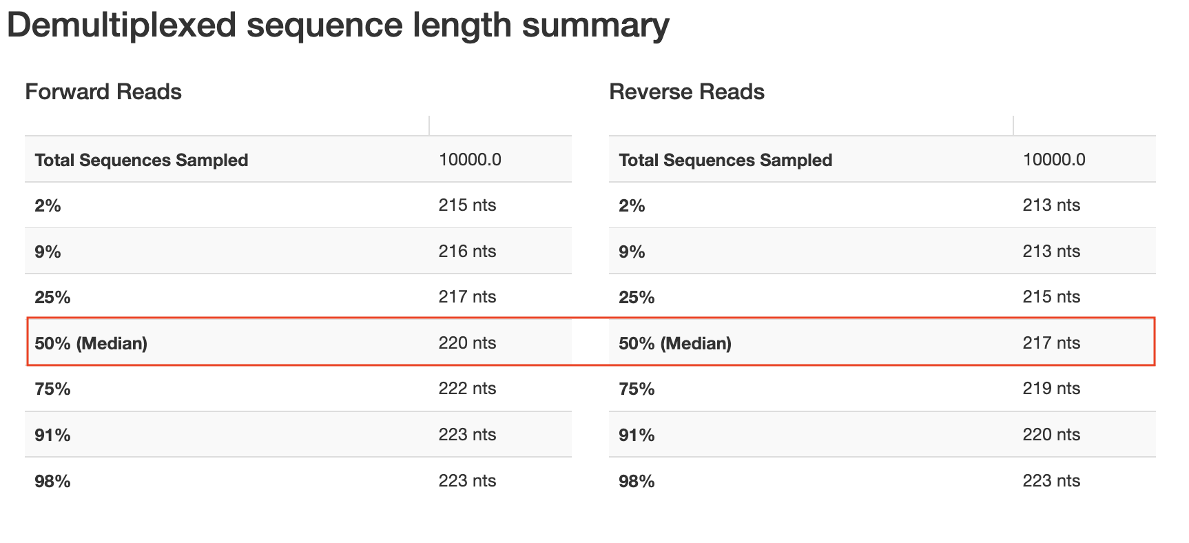
Notice that these plots are based on a subsampling of 10,000 reads, so they are simply a representation of our data. Based on these results, we will need to trim at a maximum of ~217 bp (forward) and ~215 bp (reverse) if we want to retain a majority of our sequences. In the Cancer Microbiome tutorial, they suggest truncating sequences when the twenty-fifth percentile quality score drops below 30. This is a bit conservative; I would consider lowering this to 25. The cutoffs are fairly arbitrary and will be data dependent. Normally, I would trim at ~221 bp for the forward and ~213 bp for the reverse, but due to the length inconsistencies, let's go a bit shorter to avoid losing shorter reads (207 bp Forward; 204 bp Reverse). Even with this lower cut off, our reads should overlap just fine. I will also set --p-n-threads to 2 or more to improve the speed. Threads should be set based on your computational resources.

time qiime dada2 denoise-paired \
  --i-demultiplexed-seqs demuxsequences.qza \
  --p-trunc-len-f 207 \
  --p-trunc-len-r 204 \
  --p-n-threads 2 \
  --o-representative-sequences asv-sequences.qza \
  --o-table feature-table.qza \
  --o-denoising-stats dada2-stats.qza  

(With 8 threads, this took 13 minutes, so we will run this at the beginning of the lesson.)

Denoising stats

Let's take a look at our DADA2 stats. This will give us an idea about the number of reads filtered at various steps.

qiime metadata tabulate \
  --m-input-file dada2-stats.qza \
  --o-visualization dada2-stats-summ.qzv  

Upon examining our denoising stats, we can see that > 80% of reads passed the initial input filter; 75-92% of reads were merged, and 70-92% or reads were non-chimeric. If you see heavy read loss here, you may want to refer back to your quality information and adjust denoising parameters.

Feature table and feature data summary information

Finally, we want to obtain summary information from our feature table and feature data (representative sequences). Our feature table includes count data of our ASVs in each sample, while the feature data provides the sequence for each ASV.

qiime feature-table summarize \
  --i-table feature-table.qza \
  --m-sample-metadata-file /data/sample-metadata.tsv \
  --o-visualization feature-table-summ.qzv
qiime feature-table tabulate-seqs \
  --i-data asv-sequences.qza \
  --o-visualization asv-sequences-summ.qzv  

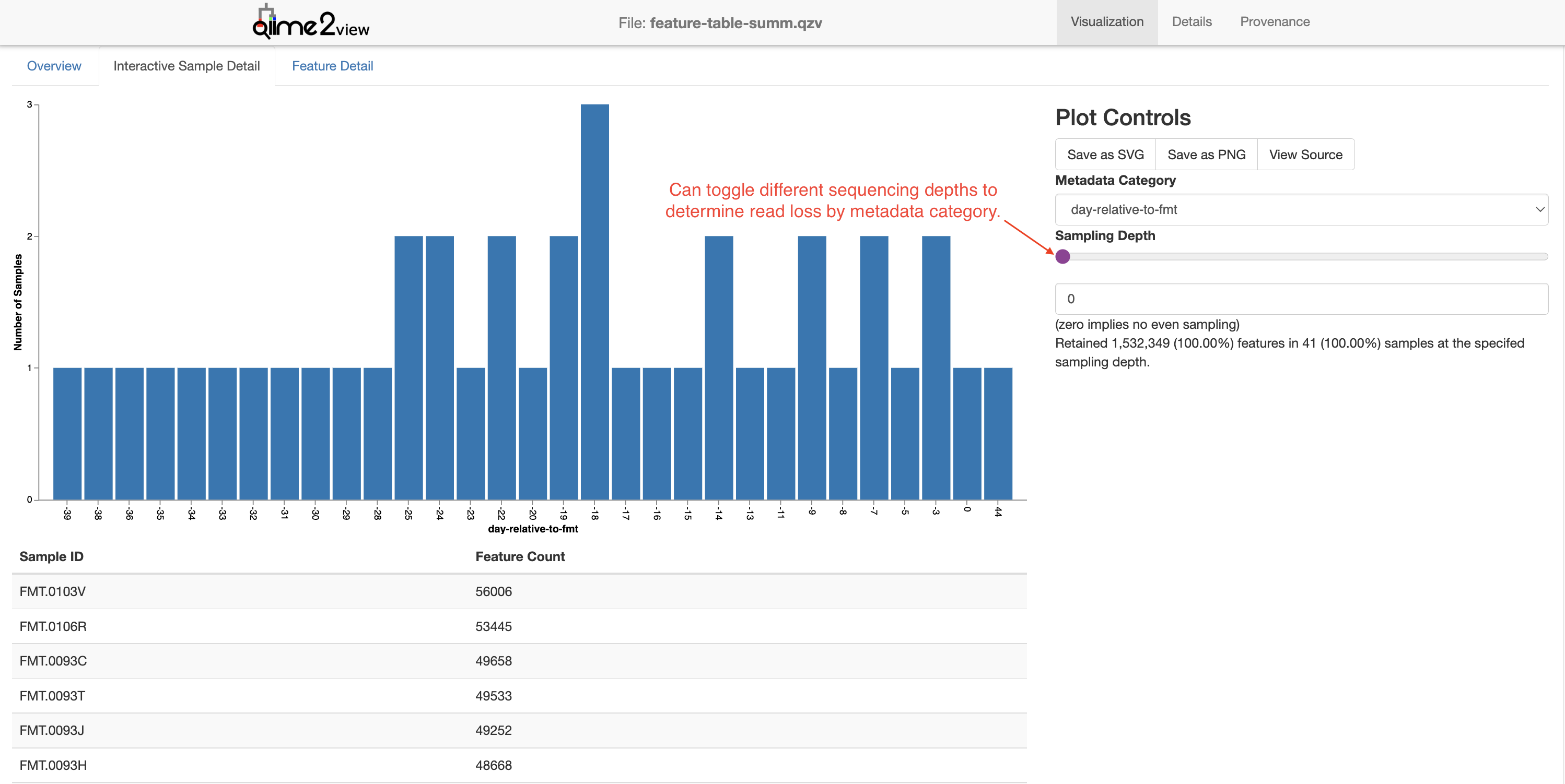
In the Interactive Sample Detail you can obtain additional information about how modifying the sequencing depth (i.e., rarefaction) impacts sample loss. (More on rarefaction later.)

We can also look at a summary of our representative sequences. Unless you modified denoising parameters, feature ids will be hashed. The hash is always the same for identical sequences, so this is not an issue for merging runs. The cool thing about this interactive summary is that you can click on the sequence, which will take you to NCBI's blastn.

We can also see that our read lengths match nicely with our expected amplicon size without primers (~330 bp).

Important note: DADA2 and Deblur are not length agnostic, meaning features with different sequencing lengths will be considered different features. Thus, we are generally fairly careful when choosing method parameters, especially if merging several sequencing runs. The same parameters should be applied across all runs. For DADA2, it is important that runs be denoised individually and then merged.

References

https://www.zymoresearch.com/blogs/blog/microbiome-informatics-otu-vs-asv www.drive5.com Elbrecht V, Vamos EE, Steinke D, Leese F. 2018. Estimating intraspecific genetic diversity from community DNA metabarcoding data. PeerJ 6:e4644 https://doi.org/10.7717/peerj.4644