Lesson 5: Microbial diversity, alpha rarefaction, alpha diversity
Learning Objectives
- Understand the difference between alpha and beta diversity
- Introduce several alpha diversity metrics
- Understand what rarefaction is and why it is important
- Introduce the debate regarding rarefaction and other methods of normalization
Often many questions related to the microbiome center on ecological diversity. How many and what types of microbes are in a sample and how does this compare to other samples? Microbial diversity is often sensitive to environmental disturbances (e.g., trauma, medication, sanitation, diet, etc.).
There are two primary types of diversity explored in microbial ecology: alpha diversity and beta diversity.
What is alpha diversity?
Alpha diversity is within sample diversity. When exploring alpha diversity, we are interested in the distribution of microbes within a sample or metadata category. This distribution not only includes the number of different organisms (richness) but also how evenly distributed these organisms are in terms of abundance (evenness).

Image modified from https://www.genome.gov/genetics-glossary/Microbiome
In addition, some diversity metrics include a phylogenetic component (i.e., Faith's phylogenetic diversity). The logic behind a phylogenetic metric is that a sample comprised of some number of highly related organisms, for example, all from the same genus, is not as diverse as a sample comprised of organisms with greater phylogenetic distances (for example, organisms from different phyla or even different domains).
Alpha diversity methods include information on either richness, evenness, or both. Here are a few examples:
Richness: High richness equals more ASVs or more phylogenetically dissimilar ASVs in the case of Faith's PD.
Observed OTUs/ASVs
Faith's PD (Sum of branch lengths)
Both: Diversity increases as richness and evenness increase.
Simpson's Dominance or Gini-Simpson (biased toward dominant species, meaning it is impacted more by evenness; values 0-1)
Shannon (treats rare and abundant more equitably than Gini-Simpson; values mostly from 0-10, typically 1-3.5)
Evenness: High values suggest more equal numbers between species.
Pileou's Evenness - calculated from Shannon (values 0-1)
Simpson's Evenness
In QIIME2, alpha diversity metrics are computed using scikit-bio; here is a link to the metrics with included descriptions.
Additionally, here is a nice resource comparing some prominent alpha diversity indices.
It is good practice to report more than one metric, since each metric can be interpreted slighlty differently.
Beta diversity (More on this in Lesson 6)
Beta diversity is between sample diversity. This is useful for answering the question, how different are these microbial communities?
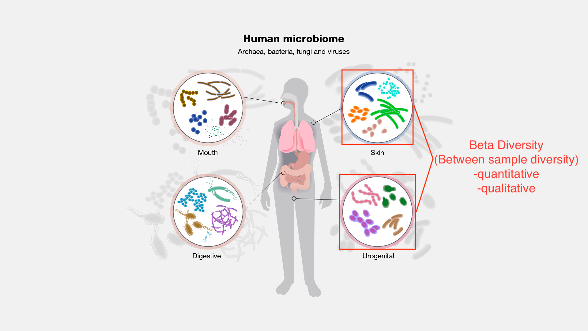
Image modified from https://www.genome.gov/genetics-glossary/Microbiome
We will look into specific metrics of beta diversity in Lesson 5.
Rarefaction
To rarefy or not to rarefy?
Feature tables are composed of sparse and compositional data. Measuring microbial diversity using 16S rRNA sequencing is dependent on sequencing depth. By chance, a sample that is more deeply sequenced is more likely to exhibit greater diversity than a sample with a low sequencing depth.
While there is a debate in the field about the most appropriate way to normalize data (See here and here) prior to downstream analyses, rarefaction is still used as a primary method for correcting differences in read depth prior to diversity analyses and is the included method used in the core diversity metrics pipeline in QIIME 2.
Note: you may want to skip rarefaction if library sizes are fairly even. Rarefaction is more beneficial when there is a greater than ~10x difference in library size (Weiss et al. 2017).
What is rarefaction?
Rarefaction is the process of subsampling reads without replacement to a defined sequencing depth, thereby creating a standardized library size across samples. Any sample with a total read count less than the defined sequencing depth used to rarefy will be discarded. Post-rarefaction all samples will have the same read depth. How do we determine the magic sequencing depth at which to rarefy? We typically use an alpha rarefaction curve.
Selecting a read depth to rarefy
A rarefaction curve
plot[s] the number of counts sampled (rarefaction depth) vs. the expected value of species diversity. --- Weiss et al. 2017
Let's take a look at an alpha rarefaction curve.
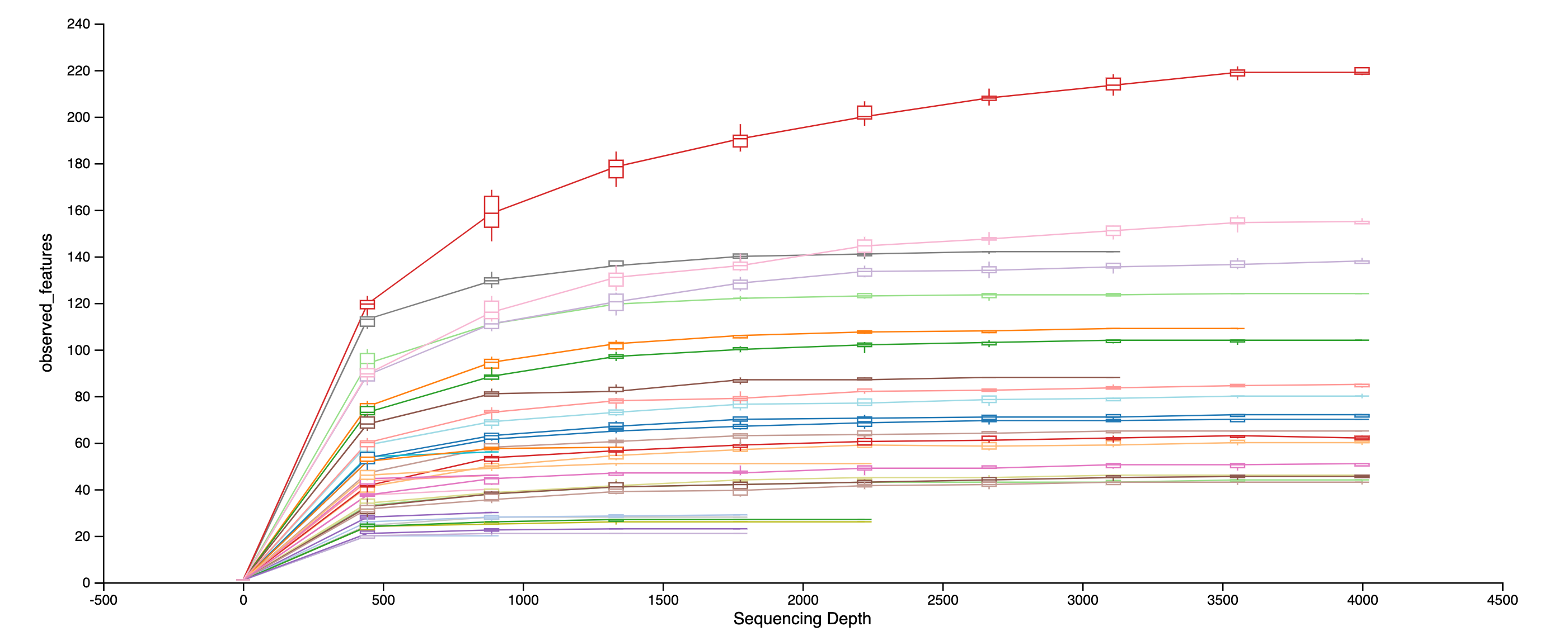
Demo plot from view.qiime2.org.
As the sequencing depth increases, you recover more and more of the diversity observed in the data. At a certain point (read depth), diversity will stabilize, meaning the diversity in the data has been fully captured. This point of stabilization will result in the diversity measure of interest plateauing.
Let's create an alpha rarefaction plot.
qiime diversity alpha-rarefaction \
  --i-table filtered-table-3.qza \
  --i-phylogeny /data/cancer_data_catchup/phylogeny-align-to-tree-mafft-fasttree/rooted_tree.qza \
  --m-metadata-file /data/sample-metadata.tsv \
  --p-max-depth 33000 \
  --o-visualization alpha-rarefaction-plot.qzv
You can adjust the metrics produced as well as other parameters regarding the number of sequencing depths to include, the minimum rarefaction depth, and the number of rarefied tables to compute at each depth (10 by default). See the help documentation for more information.
qiime diversity alpha-rarefaction --help
We can use this plot in combination with our feature table summary to decide at which depth we would like to rarefy. We need to choose a sequencing depth at which the diveristy in most of the samples has been captured and most of the samples have been retained.
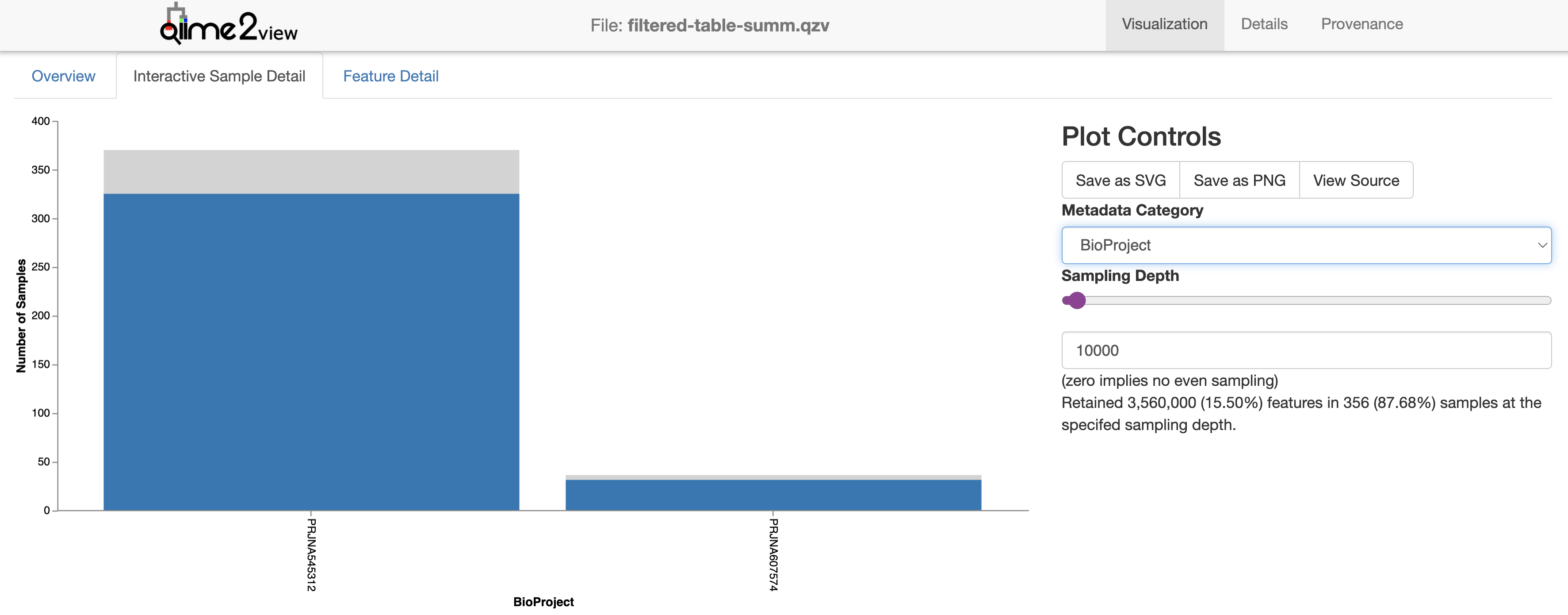
At a sampling depth of 10,000, we lose ~50 samples and retain 87% of samples, while at 15,000, we only retain ~80% of samples.
We can also check out the stability of our beta diversity metrics at a given sequencing depth using qiime diversity beta-rarefaction, which produces an "Emperor jackknifed PCoA plot, samples clustered by UPGMA or neighbor joining with support calculation, and a heatmap showing the correlation between rarefaction trials of that beta diversity metric".
Rarefying is generally applied only to diversity analyses, and many of the methods in QIIME 2 will use plugin specific normalization methods (e.g., q2-breakaway, ANCOM, ALDEx2).
Core metrics phylogenetic
We will produce a number of core diversity metrics (alpha and beta) using a QIIME 2 pipeline, qiime diversity core-metrics-phylogenetic.
The parameters we need to know include the path to our rooted tree (--i-phylogeny), the path to our feature table (--i-table), the sampling depth at which we would like to rarefy (--p-sampling-depth), the path to the sample information (--m-metadata-file), and the name of the directory we would like to save our results to (--output-dir). If you do not have a tree, or you are not interested in phylogenetic diversity metrics, you can also use qiime diversity core-metrics. We can speed up this command by including the --p-n-jobs-or-threads parameter.
qiime diversity core-metrics-phylogenetic \
  --i-phylogeny /data/cancer_data_catchup/phylogeny-align-to-tree-mafft-fasttree/rooted_tree.qza \
  --i-table filtered-table-3.qza \
  --p-sampling-depth 10000 \
  --p-n-jobs-or-threads 3 \
  --m-metadata-file /data/sample-metadata.tsv \
  --output-dir diversity-core-metrics-phylogenetic
Let's take a look at the output.
ls -l diversity-core-metrics-phylogenetic
You should see something like this:
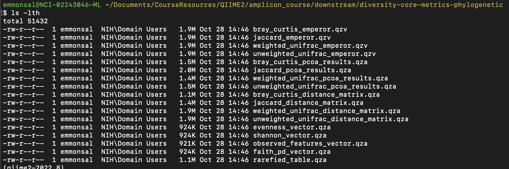
For alpha diversity, core-metrics-phylogenetic returns an evenness_vector.qza, shannon_vector.qza, observed_features_vector.qza, and faith_pd_vector.qza.
Alpha diversity comparison
Let's remember back to the design of the study we are examining (Reconstitution of the gut microbiota of antibiotic-treated patients by autologous fecal microbiota transplant).
This study included a randomized controlled longitudinal trial involving 25 patients (14 received auto-FMT following allogeneic stem cell transplanation and 11 did not). Antibiotics were given prior to the transplant to avoid serious infection, but a loss in microbial gut diversity can consequently leads to adverse health outcomes following transplantation. This study showed that auto-FMT could restore gut microbial diversity and composition to a pre-transplantation state.
To assess differences in alpha diversity by metadata category, we can use qiime diversity alpha-group-significance.
qiime diversity alpha-group-significance \
  --i-alpha-diversity diversity-core-metrics-phylogenetic/observed_features_vector.qza \
  --m-metadata-file /data/sample-metadata.tsv \
  --o-visualization alpha-group-sig-obs-feats.qzv
This reports kruskal-wallis results and kruskal-wallis pairwise results with Benjamini and Hochberg FDR corrected p-values (q-value in this case). If we are interested in assessing the relationship between an alpha diversity metric and a continuous variable, we could use qiime diversity alpha-correlation, which applies a Spearman correlation.
We notice there is a lot of variation within an individual, but because we are examining longitudinal assumptions, this type of test is inappropriate because it violates the assumption that data are independent.
Q2-longitudinal
Luckily, there is a q2-longitudinal plugin to handle dependent longitudinal data.
The q2-longitudinal plugin includes:
- interactive plotting (e.g., volatility plots)
- linear mixed effects models
- paired differences and distances
- non-metric microbial interdependence testing (NMIT)
- First differences and distances
- Supervised regression for longitudinal feature selection
For example, we can use a linear mixed effects model to better explore changes in richness related to the timing of the bone marrow transplant.
LME models examine the relationship between one or more independent variables (effects) and a single longitudinal response, where observations are made across dependent samples, e.g., in repeated-measures experiments.
The linear-mixed-effects action in q2-longitudinal uses statsmodels’ “mixedlm” function to compute LME models. --- Bokulich et al. 2018
LMEs take into account both fixed and random effects, where fixed effects are similar to factor levels and random effects represent sources of unknown variation. For example, here, we can set PatientID as a random effect; each patient has a different starting microbiome. Note: "a random intercept for each individual is set by default" (plugin description).
Check out available parameters:
qiime longitudinal linear-mixed-effects
Note: we can specify two input metadata files to merge metadata information.
Let's see how this works before we run the model.
qiime metadata tabulate \
  --m-input-file /data/sample-metadata.tsv diversity-core-metrics-phylogenetic/observed_features_vector.qza \
  --o-visualization merged_meta_alpha_summ.qzv
Let's run the LME.
qiime longitudinal linear-mixed-effects \
  --m-metadata-file /data/sample-metadata.tsv diversity-core-metrics-phylogenetic/observed_features_vector.qza \
  --p-state-column DayRelativeToNearestHCT \
  --p-individual-id-column PatientID \
  --p-metric observed_features \
  --o-visualization lme-obs-features-HCT.qzv
And, we can look at the impact of the auto-FMT.
qiime longitudinal linear-mixed-effects \
  --m-metadata-file /data/sample-metadata.tsv diversity-core-metrics-phylogenetic/observed_features_vector.qza \
  --p-state-column day-relative-to-fmt \
  --p-individual-id-column PatientID \
  --p-metric observed_features \
  --o-visualization lme-obs-features-FMT.qzv
Let's check out the qzv files produced by these commands. As always, visualization files should be moved to the ~/public directory. See the Cancer Microbiome Intervention Tutorial for a description of the results.
Optional filtering of samples
If we want to retain only the samples included in our diversity analyses, we can use qiime feature-table filter-samples to drop samples with read depths less than 10,000.
qiime feature-table filter-samples \
  --i-table filtered-table-3.qza \
  --p-min-frequency 10000 \
  --o-filtered-table filtered-table-4.qza
Note: I generally use qiime2 for upstream processing (denoising, classification, tree building) and then use R for the remainder of my analyses. R is a language and statistical computing environment, and there are many different packages that are specific to microbiome analysis (e.g., phyloseq, microbiomeSeq).