Basics of R Programming
Objectives
To understand some of the most basic features of the R language including:
- Creating R objects and understanding object types
- Using mathematical operations
- Using comparison operators
- Creating, subsetting, and modifying vectors
By the end of this section, you should understand what an object and vector is and how to access and work with objects and vectors.
R objects
Everything assigned a value in R is technically an object. Mostly we think of R objects as something in which a method (or function) can act on; however, R functions, too, are R object. R objects are what gets assigned to memory in R and are of a specific type or class. Objects include things like vectors, lists, matrices, arrays, factors, and data frames. Don't get too bogged down by terminology. Many of these terms will become clear as we begin to use them in our code. In order to be assigned to memory, an r object must be created.
Creating and deleting objects
To create an R object, you need a name, a value, and an assignment operator (e.g., <- or =). R is case sensitive, so an object with the name "FOO" is not the same as "foo".
Note
You can use alt + - on a PC to generate the -> or option + - on a mac.
Let's create a simple object and run our code. There are a few methods to run code (the run button, key shortcuts (Windows: ctrl+Enter, Mac: Command+Return), or type directly into the console).
#You can and should annotate your code with comments for better
#reproducibility.
#Create an object called "a" assigned to a value of 1.
a<-1

#Simply call the name of the object to print the value to the screen
a
## [1] 1
<- is the assignment operator.
Naming conventions and reproducibility
There are rules regarding the naming of objects.
1. Avoid spaces or special characters EXCEPT '_' and '.'
2. No numbers or underscores at the beginning of an object name.
For example:
1a<-"apples" # this will throw and error
1a
## Error: <text>:1:2: unexpected symbol
## 1: 1a
##      ^
Note
It is generally a good habit to not begin sample names with a number.
In contrast:
a<-"apples" #this works fine
a
## [1] "apples"
3. Avoid common names with special meanings (See
?Reserved) or assigned to existing functions (These will auto complete).
See the tidyverse style guide for more information on naming conventions.
How do I know what objects have been created?
To view a list of the objects you have created, use ls() or look at your global environment pane.***
Reassigning objects
To reassign an object, simply overwrite the object.
#object with gene named 'tp53'
gene_name<-"tp53"
gene_name
## [1] "tp53"
#if instead we want to reassign gene_name to a different gene,
#we would use:
gene_name<-"GH1"
gene_name
## [1] "GH1"
Warning
R will not warn you when objects are being overwritten, so use caution.
Deleting objects
# delete the object 'gene_name'
rm(gene_name)
#the object no longer exists, so calling it will result in an error
gene_name
## Error in eval(expr, envir, enclos): object 'gene_name' not found
Object data types
The data type of an R object affects how that object can be used or will behave. Examples of base R data types include numeric, integer, complex, character, and logical. R objects can also have certain assigned attributes (related to class), and these attributes will be important for how they interact with certain methods / functions. Ultimately, understanding the mode / type and class of an object will be important for how an object can be used in R. When the mode of an object is changed, we call this "coercion". You may see a coercion warning pop up when working with objects in the future.
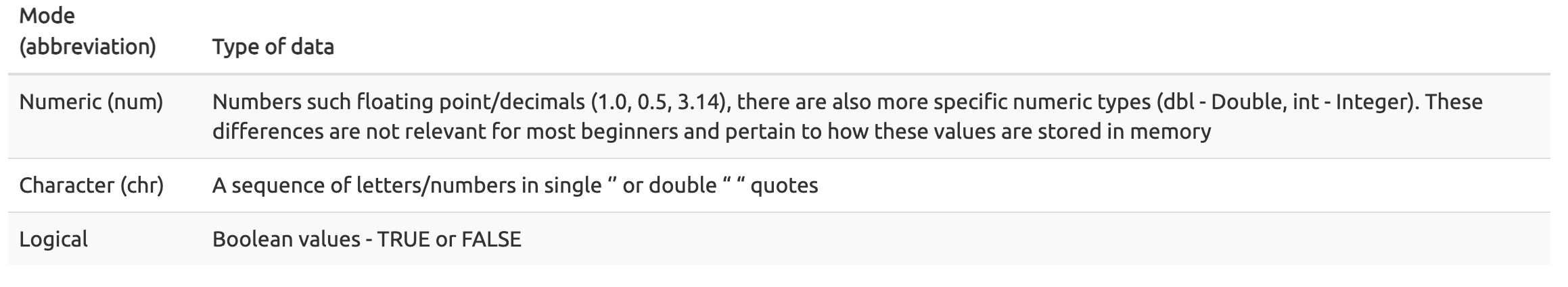
The most common modes (from datacarpentry.org); Other examples: complex, raw, etc. (See ?typeof()).
Data types are familiar in many programming languages, but also in natural language where we refer to them as the parts of speech, e.g. nouns, verbs, adverbs, etc. Once you know if a word - perhaps an unfamiliar one - is a noun, you can probably guess you can count it and make it plural if there is more than one (e.g. 1 Tuatara, or 2 Tuataras). If something is a adjective, you can usually change it into an adverb by adding “-ly” (e.g. jejune vs. jejunely). Depending on the context, you may need to decide if a word is in one category or another (e.g “cut” may be a noun when it’s on your finger, or a verb when you are preparing vegetables). These concepts have important analogies when working with R objects.
--- datacarpentry.org
The mode or type of an object can be examined using mode() or typeof(), while the class of an object can be viewed using class().
Let's create some objects and determine their types and classes.
chromosome_name <- 'chr02'
mode(chromosome_name)
## [1] "character"
typeof(chromosome_name)
## [1] "character"
class(chromosome_name)
## [1] "character"

od_600_value <- 0.47
mode(od_600_value)
## [1] "numeric"
typeof(od_600_value)
## [1] "double"
class(od_600_value)
## [1] "numeric"

df<-head(iris)
mode(df)
## [1] "list"
typeof(df)
## [1] "list"
class(df)
## [1] "data.frame"


chr_position <- '1001701bp'
mode(chr_position)
## [1] "character"
typeof(chr_position)
## [1] "character"
class(chr_position)
## [1] "character"

spock <- TRUE
mode(spock)
## [1] "logical"
typeof(spock)
## [1] "logical"
class(spock)
## [1] "logical"
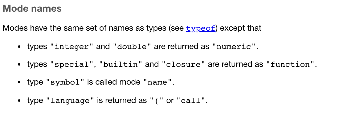
mode() and typeof() is largely the same but typeof() does differ in some cases and is based on the storage mode. So numeric types can be stored in memory differently, with doubles taking up more memory than an integer, for example. If this is confusing, you can always read the documentation ?mode() and ?typeof(). Searching for help provided this nifty R explanation for mode vs type names.
On the other hand,
'class' is a property assigned to an object that determines how generic functions operate with it. It is not a mutually exclusive classification. If an object has no specific class assigned to it, such as a simple numeric vector, it's class is usually the same as its mode, by convention. ---stackexchange
There are also functions that can gauge types directly, for example, is.numeric(), is.character(), is.logical(). It is often most useful to use class() and typeof() to find out more about an object or str() (more on this function later).
There are some special use, null-able values. Read more to learn about NULL, NA, NaN, and Inf.
Mathematical operations
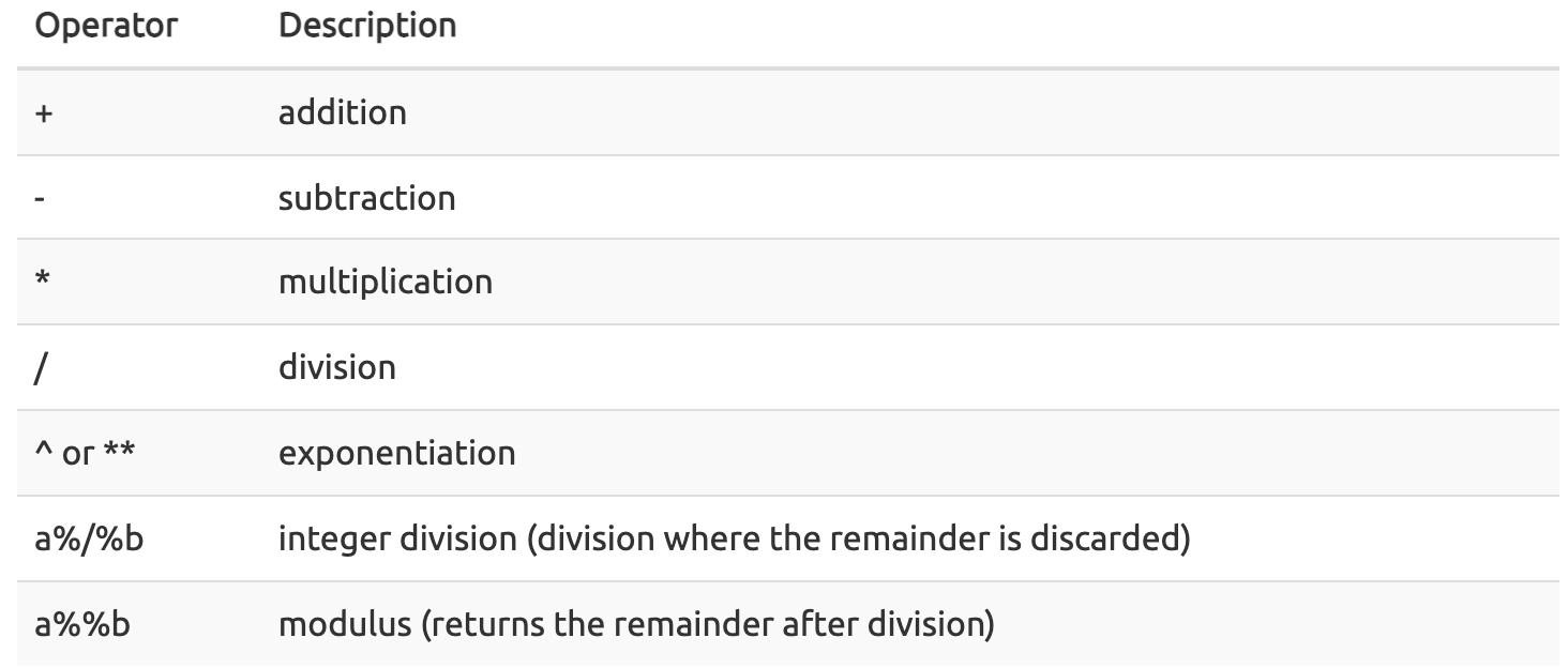
As mentioned, an object's mode can be used to understand the methods that can be applied to it. Objects of mode numeric can be treated as such, meaning mathematical operators can be used directly with those objects.
This chart from datacarpentry.org shows many of the mathematical operators used in R:
 Let's see this in practice.
#create an object storing the number of human chromosomes (haploid)
human_chr_number<-23
#let's check the mode of this object
mode(human_chr_number)
## [1] "numeric"
#Now, lets get the total number of human chromosomes (diploid)
human_chr_number * 2 #The output is 46!
## [1] 46
For example
(1 + (5 ** 0.5))/2
## [1] 1.618034
Vectors
Vectors are probably the most used commonly used object type in R. A vector is a collection of values that are all of the same type (numbers, characters, etc.). The columns that make up a data frame are vectors. One of the most common ways to create a vector is to use the
c()function - the “concatenate” or “combine” function. Inside the function you may enter one or more values; for multiple values, separate each value with a comma. --- datacarpentry.org.
#create a vector of gene names
transcript_names<-c("TSPAN6","TNMD","SCYL3","GCLC")
#Let's check out the mode. What do you think?
mode(transcript_names)
## [1] "character"
typeof(transcript_names)
## [1] "character"
length()
length(transcript_names)
## [1] 4
str(). str() will be invaluable for understanding more complicated data structures such as matrices and data frames, which will be discussed later.
str(transcript_names) #this will return properties of the object's underlying structure; in this case, the length and type
## chr [1:4] "TSPAN6" "TNMD" "SCYL3" "GCLC"
#We know this is a vector from the length but you could always check with
is.vector(transcript_names)
## [1] TRUE
Test your learning
Given the following R code:
numbers<- c("1","2.56","83","678")
What type of data is stored in this vector?
a. double
b. character
c. logical
d. complex
Solution
B
Creating, subsetting, modifying, exporting
Let's learn how to further work with vectors, including creating, sub-setting, modifying, and saving.
#Some possible RNASeq data
cell_line<- c("N052611", "N061011", "N080611", "N61311" )
sample_id <- c("SRR1039508", "SRR1039509", "SRR1039512", "SRR1039513", "SRR1039516", "SRR1039517", "SRR1039520", "SRR1039521")
transcript_counts <- c(679, 0, 467, 260,  60,   0)
#Get the second value from the vector cell_types
cell_line[2]
## [1] "N061011"
For example:
Programming languages like Fortran, MATLAB, Julia, and R start counting at 1, because that’s what human beings typically do. Languages in the C family (including C++, Java, Perl, and Python) count from 0 because that’s simpler for computers to do.---bioc-intro.
So to extract the last element in a vector, you could use the following annotation:
#retrieve the last element in the sample_id vector
sample_id[length(sample_id)]
## [1] "SRR1039521"
#retrieve the last element in the sample_id vector
sample_id[8]
## [1] "SRR1039521"
#Retrieve the second and third value from cell_types
cell_line[2:3]
## [1] "N061011" "N080611"
#Retrieve the first, fifth, and sixth values from transcript_counts
transcript_counts[c(1,5:6)]
## [1] 679 60 0
The combine function c() can be used to add an element to a vector.
#Lets add a gene to transcript_names
transcript_names<-c(transcript_names,"ANAPC10P1","ABCD1")
#The object will not be overwritten without assigning it to a name
transcript_names
## [1] "TSPAN6"    "TNMD"      "SCYL3"     "GCLC"      "ANAPC10P1" "ABCD1"
#Let's remove "SCYL3"
transcript_names<-transcript_names[-3]
transcript_names
## [1] "TSPAN6" "TNMD" "GCLC" "ANAPC10P1" "ABCD1"
#Let's rename "GCLC"
transcript_names[3]<-"NNAME"
transcript_names
## [1] "TSPAN6" "TNMD" "NNAME" "ANAPC10P1" "ABCD1"
#We can also call a value directly
#Rename "ABCD1" to "NEW"; more on this to come
transcript_names[transcript_names == "ABCD1"]  <- "NEW"
transcript_names
## [1] "TSPAN6" "TNMD" "NNAME" "ANAPC10P1" "NEW"
Logical subsetting
It is also possible to subset in R using logical evaluation or numerical comparison. To do this, we use comparison operators (See table below).
| Comparison Operator | Description |
|---|---|
| > | greater than |
| >= | greater than or equal to |
| < | less than |
| <= | less than or equal to |
| != | Not equal |
| == | equal |
| a | b | a or b |
| a & b | a and b |
So if, for example, we wanted a subset of all transcript counts greater than 260, we could use indexing combined with a comparison operator:
transcript_counts[transcript_counts > 260]
## [1] 679 467
Why does this work? Let's break down the code.
transcript_counts > 260
## [1] TRUE FALSE TRUE FALSE FALSE FALSE
This returns a logical vector. We can see that positions 1 and 3 are TRUE, meaning they are greater than 260. Therefore, the initial subsetting above is asking for a subset based on TRUE values. Here is the equivalent:
transcript_counts[c( TRUE, FALSE, TRUE, FALSE, FALSE, FALSE)]
## [1] 679 467
You can also use this functionality to do a kind of find and replace. Perhaps we want to find zero values and replace them with NAs. We could use:
transcript_counts[transcript_counts==0]<-NA
Note
if you instead ran transcript_counts[transcript_counts==0]<-"NA", you would coerce this vector to a character vector.
Now, if we want to return only values that aren't NAs, we can use
transcript_counts[!is.na(transcript_counts)] #values that aren't NAs
## [1] 679 467 260 60
is.na(transcript_counts) #if you simply want to know if there are NAs
## [1] FALSE TRUE FALSE FALSE FALSE TRUE
which(is.na(transcript_counts)) #if you want the indices of those NAs
## [1] 2 6
Other ways to handle missing data
Other functions you may find useful when working with NAs inclue na.omit() and complete.cases().
na.omit() removes the NAs from a vector.
na.omit(transcript_counts)
## [1] 679 467 260  60
## attr(,"na.action")
## [1] 2 6
## attr(,"class")
## [1] "omit"
complete.cases() creates a logical vector that you can use for subsetting based on the absence of NAs.
transcript_counts[complete.cases(transcript_counts)]
## [1] 679 467 260 60
Using objects to store thresholds
To make scripting reproducible, you could avoid calling a specific number directly and use objects in logical evaluations like those above. If we use an object, the value itself could easily be replaced with whatever value is needed. For example:
trnsc_cutoff <- 260
transcript_counts[transcript_counts>trnsc_cutoff] #note this will also include NAs in the output
## [1] 679 NA 467 NA
transcript_counts[!is.na(transcript_counts) & transcript_counts>trnsc_cutoff] #if we want to exclude possible NAs, something like this will work
## [1] 679 467
Using the %in% operator.
There may be a time you want to know whether there are specific values in your vector. To do this, we can use the %in% operator (?match()). This operator returns TRUE for any value that is in your vector and can be used for subsetting. It makes more sense to use this with data frames but we can see how this works here.
For example:
# have a look at transcript_names
transcript_names
## [1] "TSPAN6" "TNMD" "NNAME" "ANAPC10P1" "NEW"
# test to see if "NNAME" and "ANAPC10P1" are in this vector
# if you are looking for more than one value, you must pass this as a vector

c("NNAME","ANAPC10P1") %in% transcript_names
## [1] TRUE TRUE
#We could also save the search vector to an object and search that way.
find_transcripts<-c("NNAME","ANAPC10P1")
find_transcripts %in% transcript_names
## [1] TRUE TRUE
#to use this for subetting the vector lengths should match
transcript_names[transcript_names %in% find_transcripts]
## [1] "NNAME" "ANAPC10P1"
Test your learning
Given the following R code:
fruit<-c("apples", "bananas", "oranges", "grapes","kiwi","kumquat")
What does fruit[5]<-"mango" do?
a. renames the object "fruit" to "mango"
b. adds "mango" to an existing vector named "fruit"
c. replaces "bananas" with "mango"
d. replaces "kiwi" with "mango"
Solution
D
Given the following R code:
Total_subjects <- c(23, 4, 679, 3427, 12, 890, 654)
Which of the following could be used to return all values less than 678 in the vector "Total_subjects"?
a. Total_subjects < 678
b. Total_subjects[> 678]
c. Total_subjects(Total_subjects < 678)
d. Total_subjects[Total_subjects < 678]
Solution
D
Saving and loading objects
We discussed saving the R workspace (.RData), but what if we simply want to save a single object. In such a case, we can use saveRDS().
Let's save our transcript_counts vector to our working directory.
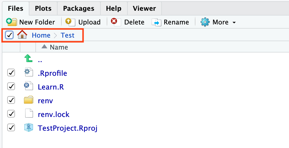
saveRDS(transcript_counts,"transcript_counts.rds")
Files pane for your newly created file. Make sure you are viewing the contents of your working directory (getwd()).
Exporting your R project
To use the materials you generated on the RServer on DNAnexus on your local computer, let's export our files. To do this, let's select all files in our working directory. This will export a zipped file with the contents of your working directory.
If you plan to use these files again on DNAnexus, simply use Upload. To upload a directory, the contents must be zipped. To zip a directory on a mac, simply right click on the directory and select Compress "directory_name". To zip a directory on a PC, right click the folder and choose "Send to: Compressed (zipped) folder".
Acknowledgments
Material from this lesson was either taken directly or adapted from the Intro to R and RStudio for Genomics lesson provided by datacarpentry.org. Material was also inspired by content from Introduction to data analysis with R and Bioconductor, which is part of the Carpentries Incubator.