Data Frames and Data Wrangling (Part 1)
This lesson will introduce data wrangling with R. Attendees will learn to filter data using base R and tidyverse (dplyr) functionality.
Learning Objectives
- Understand the concept of tidy data.
- Become familiar with the tidyverse packages.
- Be able to filter a data frame by rows and columns using base R and
dplyr.
Best Practices for organizing genomic data
Let's refer back to our best practices for organizing genomic data.
-
"Keep raw data separate from analyzed data" -- datacarpentry.org
-
"Keep spreadsheet data Tidy" -- datacarpentry.org
But, what is tidy data???
-
"Trust but verify" -- datacarpentry.org
Introducing tidy data
What is tidy data?
Tidy data is an approach (or philosophy) to data organization and management. There are three rules to tidy data: (1) each variable forms its own column, (2) each observation forms a row, and (3) each value has its own cell. One advantage to following these rules is that the data structure remains consistent, making it easier to understand the tools that work well with the underlying structure, and there are a lot of tools in R built specifically to interact with tidy data. Equipped with the right tools will make data analysis more efficient. See the infographics below.
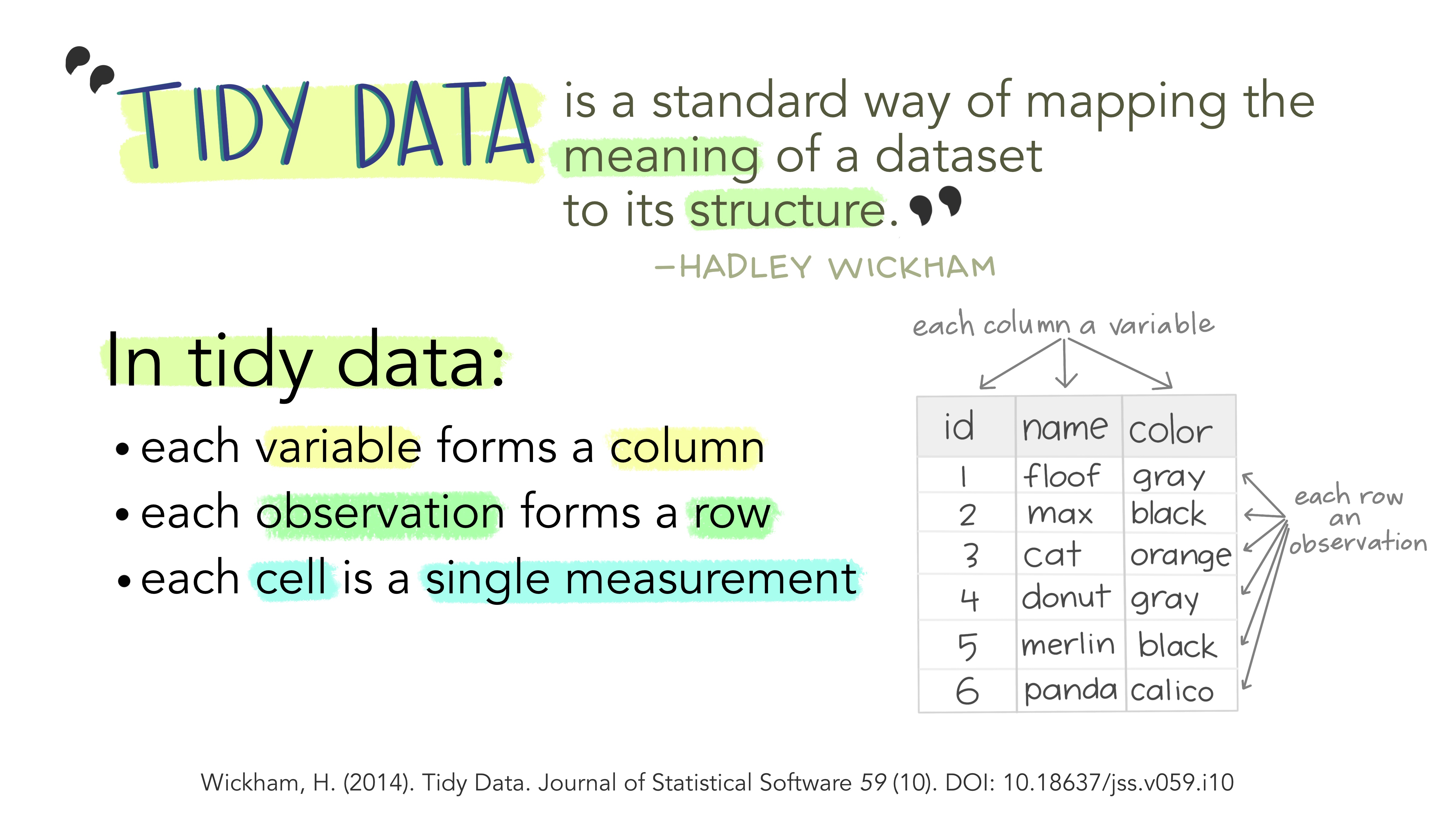
Image from Lowndes and Horst 2020: Tidy Data for Efficiency, Reproducibility, and Collaboration
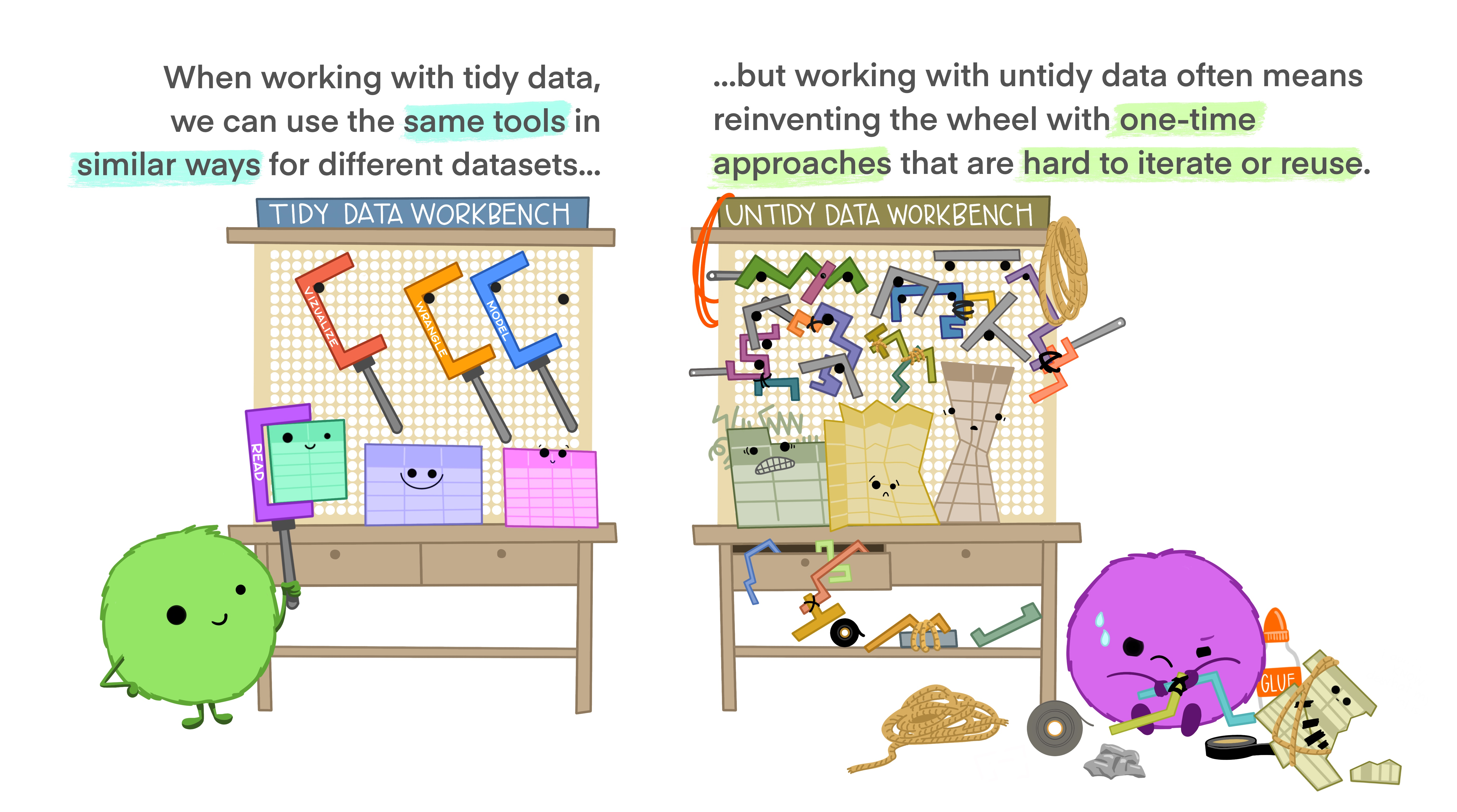
Image from Lowndes and Horst 2020: Tidy Data for Efficiency, Reproducibility, and Collaboration
What is messy data?
“Tidy datasets are all alike, but every messy dataset is messy in its own way.” –– Hadley Wickham.
Messy data sets tend to share five common problems:
- Column headers are values, not variable names.
- Multiple variables are stored in one column.
- Variables are stored in both rows and columns.
- Multiple types of observational units are stored in the same table.
- A single observational unit is stored in multiple tables. --- Hadley Wickham, Tidy Data
Let's look at a few examples of untidy data presented in Tidyverse Skills for Data Science.
Remember our data frame scaled_counts? scaled_counts is a tidy data frame. Let's take a moment to envision an untidy data frame containing the same data. Again, remember, there are infinite possibilities for messy data, but here is one example.
The orginal data frame:
#import the data and save to an object called scaled_counts
scaled_counts<-read.delim(
  "./data/filtlowabund_scaledcounts_airways.txt", as.is=TRUE)
head(scaled_counts)
          feature sample counts SampleName   cell   dex albut        Run
1 ENSG00000000003    508    679 GSM1275862 N61311 untrt untrt SRR1039508
2 ENSG00000000419    508    467 GSM1275862 N61311 untrt untrt SRR1039508
3 ENSG00000000457    508    260 GSM1275862 N61311 untrt untrt SRR1039508
4 ENSG00000000460    508     60 GSM1275862 N61311 untrt untrt SRR1039508
5 ENSG00000000971    508   3251 GSM1275862 N61311 untrt untrt SRR1039508
6 ENSG00000001036    508   1433 GSM1275862 N61311 untrt untrt SRR1039508
  avgLength Experiment    Sample    BioSample transcript ref_genome .abundant
1       126  SRX384345 SRS508568 SAMN02422669     TSPAN6       hg38      TRUE
2       126  SRX384345 SRS508568 SAMN02422669       DPM1       hg38      TRUE
3       126  SRX384345 SRS508568 SAMN02422669      SCYL3       hg38      TRUE
4       126  SRX384345 SRS508568 SAMN02422669   C1orf112       hg38      TRUE
5       126  SRX384345 SRS508568 SAMN02422669        CFH       hg38      TRUE
6       126  SRX384345 SRS508568 SAMN02422669      FUCA2       hg38      TRUE
       TMM multiplier counts_scaled
1 1.055278   1.415149     960.88642
2 1.055278   1.415149     660.87475
3 1.055278   1.415149     367.93883
4 1.055278   1.415149      84.90896
5 1.055278   1.415149    4600.65058
6 1.055278   1.415149    2027.90904
An untidy version (subset) of scaled_counts.
                                                        508
cell                                                 N61311
dex                                                   untrt
SampleName                                       GSM1275862
Run / Experiment / Accession SRR1039508;SRX384345;SRS508568
TSPAN6                                     960.886417275434
DPM1                                       660.874752382368
SCYL3                                      367.938834302817
C1orf112                                   84.9089617621886
CFH                                        4600.65057814792
                                                        509
cell                                                 N61311
dex                                                     trt
SampleName                                       GSM1275863
Run / Experiment / Accession SRR1039509;SRX384346;SRS508567
TSPAN6                                     716.779730254346
DPM1                                       823.976698841491
SCYL3                                      337.590453311757
C1orf112                                   87.9975115267612
CFH                                        5886.23354376281
                                                        512
cell                                                N052611
dex                                                   untrt
SampleName                                       GSM1275866
Run / Experiment / Accession SRR1039512;SRX384349;SRS508571
TSPAN6                                     1075.40953718585
DPM1                                       764.982041915709
SCYL3                                      323.977901809712
C1orf112                                   49.2742055984354
CFH                                        7609.16919953838
                                                        513
cell                                                N052611
dex                                                     trt
SampleName                                       GSM1275867
Run / Experiment / Accession SRR1039513;SRX384350;SRS508572
TSPAN6                                     871.667100344899
DPM1                                       779.800224573256
SCYL3                                      350.375991315107
C1orf112                                   74.7753640001752
CFH                                        9084.13850653557
                                                        516
cell                                                N080611
dex                                                   untrt
SampleName                                       GSM1275870
Run / Experiment / Accession SRR1039516;SRX384353;SRS508575
TSPAN6                                     1392.02747542151
DPM1                                       718.031746988071
SCYL3                                      299.689570719041
C1orf112                                   95.4113735350417
CFH                                        8221.28001960276
                                                        517
cell                                                N080611
dex                                                     trt
SampleName                                       GSM1275871
Run / Experiment / Accession SRR1039517;SRX384354;SRS508576
TSPAN6                                      1074.3148432507
DPM1                                       819.844851726182
SCYL3                                      339.635351591197
C1orf112                                   64.6435865566326
CFH                                        11314.6798247617
                                                        520
cell                                                N061011
dex                                                   untrt
SampleName                                       GSM1275874
Run / Experiment / Accession SRR1039520;SRX384357;SRS508579
TSPAN6                                     1212.77045557059
DPM1                                       656.786077886933
SCYL3                                      366.981189802531
C1orf112                                   119.702018991383
CFH                                        8152.33750393948
                                                        521
cell                                                N061011
dex                                                     trt
SampleName                                       GSM1275875
Run / Experiment / Accession SRR1039521;SRX384358;SRS508580
TSPAN6                                     868.672540272425
DPM1                                       771.478409892293
SCYL3                                      347.772747766408
C1orf112                                   91.1194972313732
CFH                                        12141.6730060805
Tools for working with tidy data
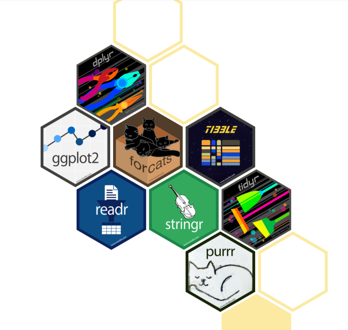
The
tidyverseis an opinionated collection of R packages designed for data science. All packages share an underlying design philosophy, grammar, and data structures. ---tidyverse.org
The core packages within tidyverse include dplyr, ggplot2, forcats, tibble, readr, stringr, tidyr, and purr, some of which we will use in this lesson and future lessons.
Load the core tidyverse packages
The tidyverse includes a collection of packages. To use these packages, we need to load the packages using the library() function.
library(tidyverse)
Load the data
To explore tidyverse functionality, let's read in some data and take a look.
#let's use our differential expression results
dexp<-readRDS("./data/diffexp_results_edger_airways.rds")
str(), but let's check out the tidyverse equivalent, glimpse().
str(dexp, give.attr=FALSE)
tibble [15,926 × 10] (S3: tbl_df/tbl/data.frame)
 $ feature   : chr [1:15926] "ENSG00000000003" "ENSG00000000419" "ENSG00000000457" "ENSG00000000460" ...
 $ albut     : Factor w/ 1 level "untrt": 1 1 1 1 1 1 1 1 1 1 ...
 $ transcript: chr [1:15926] "TSPAN6" "DPM1" "SCYL3" "C1orf112" ...
 $ ref_genome: chr [1:15926] "hg38" "hg38" "hg38" "hg38" ...
 $ .abundant : logi [1:15926] TRUE TRUE TRUE TRUE TRUE TRUE ...
 $ logFC     : num [1:15926] -0.3901 0.1978 0.0292 -0.1244 0.4173 ...
 $ logCPM    : num [1:15926] 5.06 4.61 3.48 1.47 8.09 ...
 $ F         : num [1:15926] 32.8495 6.9035 0.0969 0.3772 29.339 ...
 $ PValue    : num [1:15926] 0.000312 0.028062 0.762913 0.554696 0.000463 ...
 $ FDR       : num [1:15926] 0.00283 0.07701 0.84425 0.68233 0.00376 ...
glimpse(dexp)
Rows: 15,926
Columns: 10
$ feature    <chr> "ENSG00000000003", "ENSG00000000419", "ENSG00000000457", "E…
$ albut      <fct> untrt, untrt, untrt, untrt, untrt, untrt, untrt, untrt, unt…
$ transcript <chr> "TSPAN6", "DPM1", "SCYL3", "C1orf112", "CFH", "FUCA2", "GCL…
$ ref_genome <chr> "hg38", "hg38", "hg38", "hg38", "hg38", "hg38", "hg38", "hg…
$ .abundant  <lgl> TRUE, TRUE, TRUE, TRUE, TRUE, TRUE, TRUE, TRUE, TRUE, TRUE,…
$ logFC      <dbl> -0.390100222, 0.197802179, 0.029160865, -0.124382022, 0.417…
$ logCPM     <dbl> 5.059704, 4.611483, 3.482462, 1.473375, 8.089146, 5.909668,…
$ F          <dbl> 3.284948e+01, 6.903534e+00, 9.685073e-02, 3.772134e-01, 2.9…
$ PValue     <dbl> 0.0003117656, 0.0280616149, 0.7629129276, 0.5546956332, 0.0…
$ FDR        <dbl> 0.002831504, 0.077013489, 0.844247837, 0.682326613, 0.00376…
We can see that glimpse() is a little more succinct and clean and that str() will show attributes. These attribues were ignored above using give.attr=FALSE to get around package dependencies.
sscaled
We will also use a subset version of scaled_counts that includes the columns "sample, "cell", "dex", "transcript", "counts", and "counts_scaled".
  scaled_counts[
    c("sample","cell","dex","transcript","counts","counts_scaled")]
We can use import functions from the tidyverse to load sscaled, which are a bit more efficient and create a data frame like object, known as a tibble.
#import sscaled
sscaled<-read_delim("data/sscaled.txt")
Rows: 127408 Columns: 6
── Column specification ────────────────────────────────────────────────────────
Delimiter: "\t"
chr (3): cell, dex, transcript
dbl (3): sample, counts, counts_scaled

ℹ Use `spec()` to retrieve the full column specification for this data.
ℹ Specify the column types or set `show_col_types = FALSE` to quiet this message.
sscaled
# A tibble: 127,408 × 6
   sample cell   dex       transcript counts counts_scaled
    <dbl> <chr>  <chr>     <chr>       <dbl>         <dbl>
 1    508 N61311 untreated TSPAN6        679         961.
 2    508 N61311 untreated DPM1          467         661.
 3    508 N61311 untreated SCYL3         260         368.
 4    508 N61311 untreated C1orf112       60          84.9
 5    508 N61311 untreated CFH          3251        4601.
 6    508 N61311 untreated FUCA2        1433        2028.
 7    508 N61311 untreated GCLC          519         734.
 8    508 N61311 untreated NFYA          394         558.
 9    508 N61311 untreated STPG1         172         243.
10    508 N61311 untreated NIPAL3       2112        2989.
# ℹ 127,398 more rows
Notice the tibble output. Tibbles easily show you the data types in each column and limit output to the screen (i.e., first 10 rows; only the columns that fit). They also do not force syntactic variable names.
Subsetting data frames with base R
Before diving into subsetting with dplyr, let's take a step back and learn to subset with base R. Subsetting a data frame is similar to subsetting a vector; we can use bracket notation []. However, a data frame is two dimensional with both rows and columns, so we can specify either one argument or two arguments (e.g., df[row,column]) depending. If you provide one argument, columns will be assumed. This is because a data frame has characteristics of both a list and a matrix.
For now, let's focus on providing two arguments to subset. (Note when a df structure is returned)
scaled_counts[2,4] #Returns the value in the 4th column and 2nd row

scaled_counts[2, ] #Returns a df with row two

scaled_counts[-1, ] #Returns a df without row 1

scaled_counts[1:4,1] #returns a vector of rows 1-4 of column 1

#call names of columns directly
scaled_counts[1:10,c("sample","counts")]

#use comparison operators
scaled_counts[scaled_counts$sample == "508",]
What happens when we provide a single argument?
#notice the difference here
scaled_counts[,2] #returns column two
#treated similar to a matrix
#does not return a df if the output is a single column

scaled_counts[2] #returns column two
#treated similar to a list; maintains the df structure

#You can preserve the structure of the data frame while subsetting
# use drop = F
scaled_counts[,2,drop=F]
Note
We can also use [[]] or $ for selecting specific columns.
Using %in%
%in% "returns a logical vector indicating if there is a match or not for its left operand". This logical vector can then be used to filter the datamframe to only matched values.
For example, perhaps we have 4 transcripts that we are interested in exploring further. We can assign those transcripts to a vector.
keep_t<-c("CPD","EXT1","MCL1","LASP1")
We can then see where those transcripts match transcripts in sscaled$trasncript.
head(sscaled$transcript %in% keep_t)
[1] FALSE FALSE FALSE FALSE FALSE FALSE
We can further use this logical transcript to filter our data frame by true values.
#Let's filter our data to only include 4 transcripts of interest
interesting_trnsc<-sscaled[sscaled$transcript %in% keep_t,]
Tips to remember for subsetting
- Typically provide two values separated by commas: data.frame[row, column]
- In cases where you are taking a continuous range of numbers use a colon between the numbers (start:stop, inclusive)
- For a non continuous set of numbers, pass a vector using c()
- Index using the name of a column(s) by passing them as vectors using c() ---datacarpentry.org
Info
Subsetting including simplifying vs preserving can get confusing. Here is a great chapter - though, a bit more advanced - that may clear things up if you are confused.
Data wrangling with tidyverse
While bracket notation is useful, it is not always the most readable or easy to employ, especially for beginners. This is where dplyr comes in. The dplyr package in the tidyverse world simplifies data wrangling with easy to employ and easy to understand functions specific for data manipulation in data frames.
The package dplyr is a fairly new (2014) package that tries to provide easy tools for the most common data manipulation tasks. It was built to work directly with data frames. The thinking behind it was largely inspired by the package plyr which has been in use for some time but suffered from being slow in some cases. dplyr addresses this by porting much of the computation to C++. An additional feature is the ability to work with data stored directly in an external database. The benefits of doing this are that the data can be managed natively in a relational database, queries can be conducted on that database, and only the results of the query returned. This addresses a common problem with R in that all operations are conducted in memory and thus the amount of data you can work with is limited by available memory. The database connections essentially remove that limitation in that you can have a database that is over 100s of GB, conduct queries on it directly and pull back just what you need for analysis in R. --- datacarpentry.com
We do not need to load the dplyr package, as it is included in library(tidyverse), which we have already installed and loaded. However, if you need to install and load on your local machine you would use the following:
install.packages("dplyr")
library("dplyr")
Subsetting with dplyr
We've seen how to select columns and rows using base R, but now let's look at a more intuitive way with functions (select() and filter()) from the tidyverse package dplyr.
Selecting columns
select() requires the data frame followed by the columns that we want to select or deselect as arguments.
#select the gene / transcript, logFC, and FDR corrected p-value
#first argument is the df followed by columns to select
dexp_s<-select(dexp, transcript, logFC, FDR)
We can also select all columns, leaving out ones that do not interest us using - or !. This is helpful if the columns to keep far outweigh those to exclude.
df_exp<-select(dexp, -feature)
For readability we should move the transcript column to the front. We can select a range of columns using the :.
#you can reorder columns and call a range of columns using select().
df_exp<-select(df_exp, transcript:FDR,albut)
#Note: this also would have excluded the feature column
We can also include helper functions such as starts_with() and ends_with(). See more helper functions with ?select().
select(df_exp, transcript, starts_with("log"), FDR)
# A tibble: 15,926 × 4
   transcript   logFC logCPM     FDR
   <chr>        <dbl>  <dbl>   <dbl>
 1 TSPAN6     -0.390    5.06 0.00283
 2 DPM1        0.198    4.61 0.0770
 3 SCYL3       0.0292   3.48 0.844
 4 C1orf112   -0.124    1.47 0.682
 5 CFH         0.417    8.09 0.00376
 6 FUCA2      -0.250    5.91 0.0186
 7 GCLC       -0.0581   4.84 0.794
 8 NFYA       -0.509    4.13 0.00126
 9 STPG1      -0.136    3.12 0.478
10 NIPAL3     -0.0500   7.04 0.695
# ℹ 15,916 more rows
Test your learning
-
From the
interesting_trnscdata frame select the following columns and save to an object: sample, dex, transcript, counts_scaled.Possible Solution
interesting_trnsc_s<- select(interesting_trnsc, sample, dex, transcript, counts_scaled) -
From the
interesting_trnscdata frame select all columns except cell and counts.Possible Solution
interesting_trnsc_s2<-select(interesting_trnsc,!c(cell,counts))
Filtering by row
Now let's filter the rows based on a condition. Let's look at only the treated samples in scaled_counts using the function filter(). filter() requires the df as the first argument followed by the filtering conditions.
filter(sscaled, dex == "treated") #we've seen == notation before
We can also filter using %in%
#filter for two cell lines
f_sscale<-filter(sscaled,cell %in% c("N061011", "N052611"))
#let's check that this worked
levels(factor(f_sscale$cell))
[1] "N052611" "N061011"
#let's filter by keep_t from above
filter(f_sscale,transcript %in% keep_t)
# A tibble: 16 × 6
   sample cell    dex       transcript counts counts_scaled
    <dbl> <chr>   <chr>     <chr>       <dbl>         <dbl>
 1    512 N052611 untreated LASP1        7831         9647.
 2    512 N052611 untreated CPD          8270        10187.
 3    512 N052611 untreated MCL1         5170         6369.
 4    512 N052611 untreated EXT1         8503        10474.
 5    513 N052611 treated   LASP1        5809        12411.
 6    513 N052611 treated   CPD          7638        16318.
 7    513 N052611 treated   MCL1         5153        11009.
 8    513 N052611 treated   EXT1         2317         4950.
 9    520 N061011 untreated LASP1        5766         9082.
10    520 N061011 untreated CPD          7067        11131.
11    520 N061011 untreated MCL1         4410         6946.
12    520 N061011 untreated EXT1         6925        10907.
13    521 N061011 treated   LASP1        7825        11884.
14    521 N061011 treated   CPD         10091        15325.
15    521 N061011 treated   MCL1         7338        11144.
16    521 N061011 treated   EXT1         3242         4923.
And we can filter using numeric columns. There are lots of options for filtering so explore the functionality a bit when you get a chance.
#get only results from counts greater than or equal to 20k
#use head to get only the first handful of rows
head(filter(f_sscale,counts_scaled >= 20000))
# A tibble: 6 × 6
  sample cell    dex       transcript counts counts_scaled
   <dbl> <chr>   <chr>     <chr>       <dbl>         <dbl>
1    512 N052611 untreated CSDE1       19863        24468.
2    512 N052611 untreated MRC2        23978        29537.
3    512 N052611 untreated DCN        422752       520769.
4    512 N052611 untreated VIM         37558        46266.
5    512 N052611 untreated CD44        25453        31354.
6    512 N052611 untreated VCL         17309        21322.
#use `|` operator
#look at only results with named genes (not NAs)
#and those with a log fold change greater than 2
#and either a p-value or an FDR corrected p_value < or = to 0.01
#The comma acts as &
sig_annot_transcripts<-
  filter(df_exp, !is.na(transcript),
         abs(logFC) > 2, (PValue | FDR <= 0.01))
Test your learning
Filter the interesting_trnsc data frame to only include the following genes: MCL1 and EXT1.
Possible Solution
interesting_trnsc_f<-filter(interesting_trnsc, transcript %in% c("MCL1","EXT1"))

interesting_trnsc_f<-filter(interesting_trnsc, transcript == "MCL1" | transcript =="EXT1")
Acknowledgements
Material from this lesson was either taken directly or adapted from the Intro to R and RStudio for Genomics lesson provided by datacarpentry.org and from a 2021 workshop entitled Introduction to Tidy Transciptomics by Maria Doyle and Stefano Mangiola. This lesson was also inspired by material from "Manipulating and analyzing data with dplyr", Introduction to data analysis with R and Bioconductor.