Data Frames and Data Wrangling (Part 2)
In this lesson, attendees will learn how to transform, summarize, and reshape data using functions from the tidyverse.
Learning Objectives
Continue to wrangle data using tidyverse functionality. To this end, you should understand:
- how to use common dplyr functions (e.g.,
group_by(),arrange(),mutate(), andsummarize()). - how to employ the pipe (
|>) operator to link functions. - how to perform more complicated wrangling using the split, apply, combine concept.
- how to tidy (reshape) data using
tidyr.
Load the tidyverse
library(tidyverse)
Remember that this loads the core tidyverse packages. There are other packages that you may be interested in; see here.
Re-load the data
We will continue working with the airway data for this lesson. Let's import the data.
scaled_counts<-read_delim(
  "./data/filtlowabund_scaledcounts_airways.txt")

sscaled <- select(scaled_counts, sample,
  cell, dex, transcript, counts, counts_scaled)

dexp <- read_delim("./data/diffexp_results_edger_airways.txt")
Introducing the pipe
Often we will apply multiple functions to wrangle a data frame into the state that we need it. For example, maybe you want to select and filter. What are our options?
We could run one step after another, saving an object for each step.
Running code one step at a time
#Run one step at a time with intermediate objects.
#We've done this a few times above
#select gene, logFC, FDR
dexp_s<-select(dexp, transcript, logFC, FDR)

#Now filter for only the genes "TSPAN6" and DPM1
tspanDpm<- filter(dexp_s, transcript == "TSPAN6" | transcript=="DPM1")

#Print
tspanDpm
# A tibble: 2 × 3
  transcript  logFC     FDR
  <chr>       <dbl>   <dbl>
1 TSPAN6     -0.390 0.00283
2 DPM1        0.198 0.0770
Or we could nest a function within a function.
Nesting code
#Nested code example; processed from inside out
tspanDpm<- filter(select(dexp, c(transcript, logFC, FDR)),
                  transcript == "TSPAN6" | transcript=="DPM1" )
tspanDpm
# A tibble: 2 × 3
  transcript  logFC     FDR
  <chr>       <dbl>   <dbl>
1 TSPAN6     -0.390 0.00283
2 DPM1        0.198 0.0770
But, these affect code readability and clutter our work space, making it difficult to follow what we or someone else did.
Using the Pipe
Let's explore how piping streamlines this. Piping (using |>) allows you to employ multiple functions consecutively, while improving readability. The output of one function is passed directly to another without storing the intermediate steps as objects. You can pipe from the beginning (reading in the data) all the way to plotting without storing the data or intermediate objects, if you want.
The magrittr pipe (%>%)
Prior to R version 4.1.0, the native R pipe did NOT exist. Use of the pipe came from the magrittr package, which is a dependency of the tidyverse. While the native pipe (|>) and the magrittr pipe (%>%) are fairly similar. They are not identical. You can read more about the differences here.
To pipe, we have to first call the data and then pipe it into a function. The output of each step is then piped into the next step.
Let's see how this works
tspanDpm <- dexp |> #call the data and pipe to select()
  select(transcript, logFC, FDR) |> #select columns of interest
  filter(transcript == "TSPAN6" | transcript=="DPM1" ) #filter
tspanDpm
# A tibble: 2 × 3
  transcript  logFC     FDR
  <chr>       <dbl>   <dbl>
1 TSPAN6     -0.390 0.00283
2 DPM1        0.198 0.0770
Notice that the data argument has been dropped from select() and filter(). This is because the pipe passes the object from the left to the right.
Important
The |> must be at the end of each line.
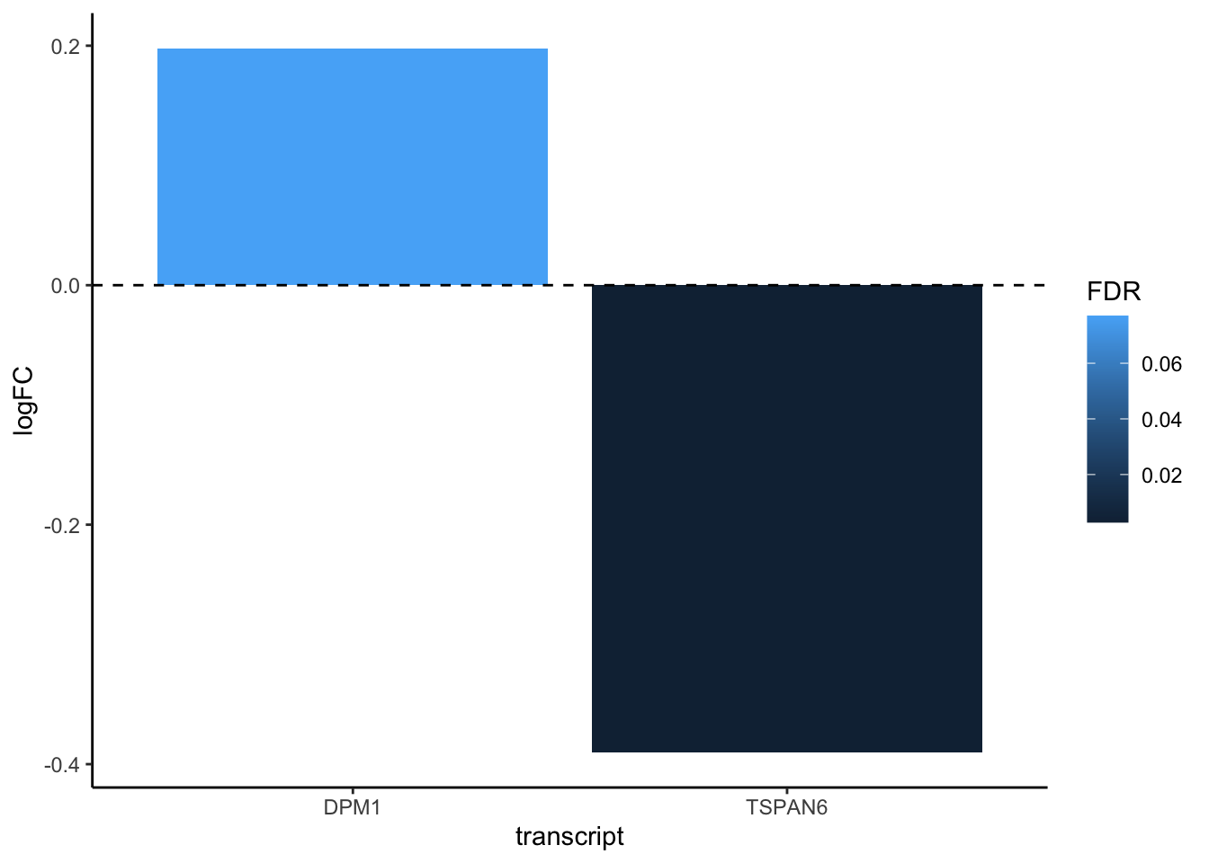
We can pipe from the beginning to the end.
readRDS("./data/diffexp_results_edger_airways.rds") |> #read data
  select(transcript, logFC, FDR) |> #select columns of interest
  filter(transcript == "TSPAN6" | transcript=="DPM1" ) |> #filter
  ggplot(aes(x=transcript,y=logFC,fill=FDR)) + #plot
  geom_bar(stat = "identity") +
  theme_classic() +
  geom_hline(yintercept=0, linetype="dashed", color = "black")
The dplyr functions by themselves are somewhat simple, but by combining them into linear workflows with the pipe, we can accomplish more complex manipulations of data frames. ---datacarpentry.org
Test your learning
Using what you have learned about select() and filter(), use the pipe (|>) to create a subset data frame from scaled_counts that only includes the columns 'sample', 'cell', 'dex', 'transcript', and 'counts_scaled' and only rows that include the treatment "untrt" and the transcripts "ACTN1" and "ANAPC4"?
Possible Solution
scaled_counts |> select(sample,cell,dex,transcript,counts_scaled) |>
  filter(dex=="untrt", transcript %in% c("ACTN1","ANAPC4"))
Mutate
Another useful data manipulation function from dplyr is mutate(). mutate() allows you to create a new variable from existing variables. Perhaps you want to know the ratio of two columns or convert the units of a variable. That can be done with mutate().
mutate()creates new columns that are functions of existing variables. It can also modify (if the name is the same as an existing column) and delete columns (by setting their value to NULL). --- dplyr.tidyverse.org
Create a new column using existing columns
Let's create a column in our original differential expression data frame denoting significant transcripts (those with an FDR corrected p-value less than 0.05 and a log fold change greater than or equal to 2).
dexp_sigtrnsc<-dexp |> mutate(Significant= FDR<0.05 & abs(logFC) >=2)
head(dexp_sigtrnsc["Significant"])
# A tibble: 6 × 1
  Significant
  <lgl>
1 FALSE
2 FALSE
3 FALSE
4 FALSE
5 FALSE
6 FALSE
The conditional evaluates to a logical vector, containing TRUE or FALSE values.
Coerce variables
We can also use mutate to coerce variables.
To mutate across multiple columns, we need to use the function across() with the select helper where().
#view sscaled
glimpse(sscaled)
Rows: 127,408
Columns: 6
$ sample        <dbl> 508, 508, 508, 508, 508, 508, 508, 508, 508, 508, 508, 5…
$ cell          <chr> "N61311", "N61311", "N61311", "N61311", "N61311", "N6131…
$ dex           <chr> "untrt", "untrt", "untrt", "untrt", "untrt", "untrt", "u…
$ transcript    <chr> "TSPAN6", "DPM1", "SCYL3", "C1orf112", "CFH", "FUCA2", "…
$ counts        <dbl> 679, 467, 260, 60, 3251, 1433, 519, 394, 172, 2112, 524,…
$ counts_scaled <dbl> 960.88642, 660.87475, 367.93883, 84.90896, 4600.65058, 2…
#use mutate with across and select helpers
ex_coerce<-sscaled |> mutate(across(where(is.character),as.factor))
glimpse(ex_coerce)
Rows: 127,408
Columns: 6
$ sample        <dbl> 508, 508, 508, 508, 508, 508, 508, 508, 508, 508, 508, 5…
$ cell          <fct> N61311, N61311, N61311, N61311, N61311, N61311, N61311, …
$ dex           <fct> untrt, untrt, untrt, untrt, untrt, untrt, untrt, untrt, …
$ transcript    <fct> TSPAN6, DPM1, SCYL3, C1orf112, CFH, FUCA2, GCLC, NFYA, S…
$ counts        <dbl> 679, 467, 260, 60, 3251, 1433, 519, 394, 172, 2112, 524,…
$ counts_scaled <dbl> 960.88642, 660.87475, 367.93883, 84.90896, 4600.65058, 2…
Note
across() has superseded the use of mutate_if, _at, _all. For more information on across() see this reference article.
More examples
Check out more examples using mutate() here
Test your learning
Using mutate apply a base 10 logarithmic transformation to the counts_scaled column of sscaled. Save the resulting data frame to an object
called log10counts. Hint: see the function log10().
Possible Solution
log10counts<-sscaled |> mutate(logCounts=log10(counts_scaled))
Arrange, group_by, summarize
There is an approach to data analysis known as "split-apply-combine", in which the data is split into smaller components, some type of analysis is applied to each component, and the results are combined. The dplyr functions including group_by() and summarize() are key players in this type of workflow. The function arrange() may also be handy.
group_by() allows us to group a data frame by a categorical variable so that a given operation can be performed per group.
Let's get the median counts_scaled by transcript within a treatment. When you reduce the size of a data set through a calculation, you need to use summarize().
scaled_counts |> #Call the data
  group_by(dex,transcript) |> # group_by treatment and transcript
  #(transcript nested within treatment)
  summarize(median_counts=median(counts_scaled))
`summarise()` has grouped output by 'dex'. You can override using the `.groups`
argument.
# A tibble: 29,152 × 3
# Groups:   dex [2]
   dex   transcript median_counts
   <chr> <chr>              <dbl>
 1 trt   A1BG-AS1            80.2
 2 trt   A2M              37821.
 3 trt   A2M-AS1             24.2
 4 trt   A4GALT            2043.
 5 trt   AAAS              1086.
 6 trt   AACS               481.
 7 trt   AADAT              154.
 8 trt   AAGAB              984.
 9 trt   AAK1               399.
10 trt   AAMDC              181.
# ℹ 29,142 more rows
The output is a grouped data frame.
Note
group_by() can also be used with mutate().
Using arrange()
Now, if we want the top five transcripts with the greatest median scaled counts by treatment, we need to organize our data frame and then return the top rows. We can use arrange() to arrange our data frame by median_counts. If we want to arrange from highest to lowest value, we will additionally need to use desc(). The .by_group allows us to arrange by median counts within a grouping. By including slice_head() we can return the top five values by group.
scaled_counts |> #Call the data
  group_by(dex,transcript) |> # group_by treatment and transcript
  #(transcript nested within treatment)
  summarize(median_counts=median(counts_scaled)) |> #for each group
  #calculate the median value of scaled counts
  arrange(desc(median_counts),.by_group = TRUE) |>
  #arrange in descending order
  slice_head(n=5) #return the top 5 values for each group
`summarise()` has grouped output by 'dex'. You can override using the `.groups`
argument.
# A tibble: 10 × 3
# Groups:   dex [2]
   dex   transcript median_counts
   <chr> <chr>              <dbl>
 1 trt   FN1              486430.
 2 trt   DCN              389306.
 3 trt   MT-CO1           369456.
 4 trt   EEF1A1           346869.
 5 trt   QSOX1            284100.
 6 untrt FN1              456360.
 7 untrt DCN              439781.
 8 untrt EEF1A1           404269.
 9 untrt MT-CO1           346974.
10 untrt COL1A2           331816.
The slice functions
We could have skipped arrange() and used slice_max(). slice_max() returns the rows with the greatest values from each group.
scaled_counts |>
  group_by(dex,transcript) |>
  summarize(median_counts=median(counts_scaled))  |>
  slice_max(median_counts, n=5) #notice use of slice_max
`summarise()` has grouped output by 'dex'. You can override using the `.groups`
argument.
# A tibble: 10 × 3
# Groups:   dex [2]
   dex   transcript median_counts
   <chr> <chr>              <dbl>
 1 trt   FN1              486430.
 2 trt   DCN              389306.
 3 trt   MT-CO1           369456.
 4 trt   EEF1A1           346869.
 5 trt   QSOX1            284100.
 6 untrt FN1              456360.
 7 untrt DCN              439781.
 8 untrt EEF1A1           404269.
 9 untrt MT-CO1           346974.
10 untrt COL1A2           331816.
The other slice functions include:
slice_head(n = 1) takes the first row from each group.
slice_tail(n = 1) takes the last row in each group.
slice_min(x, n = 1) takes the row with the smallest value of column x.
slice_sample(n = 1) takes one random row. --- R4DS.
Sample sizes (counts and tallies) and missing data
How many rows per sample are in the scaled_counts data frame?
scaled_counts  |>
  group_by(dex, sample) |>
  summarize(n=n()) #there are multiple functions that can be used here
`summarise()` has grouped output by 'dex'. You can override using the `.groups`
argument.
# A tibble: 8 × 3
# Groups:   dex [2]
  dex   sample     n
  <chr>  <dbl> <int>
1 trt      509 15926
2 trt      513 15926
3 trt      517 15926
4 trt      521 15926
5 untrt    508 15926
6 untrt    512 15926
7 untrt    516 15926
8 untrt    520 15926
#See count(); can also use tally()
scaled_counts |>
  count(dex,sample)
# A tibble: 8 × 3
  dex   sample     n
  <chr>  <dbl> <int>
1 trt      509 15926
2 trt      513 15926
3 trt      517 15926
4 trt      521 15926
5 untrt    508 15926
6 untrt    512 15926
7 untrt    516 15926
8 untrt    520 15926
Note
By default, all [built in] R functions operating on vectors that contain missing data will return NA. It’s a way to make sure that users know they have missing data, and make a conscious decision on how to deal with it. When dealing with simple statistics like the mean, the easiest way to ignore NA (the missing data) is to use
na.rm = TRUE(rm stands for remove). ---datacarpentry.org
Let's see this in practice
set.seed(138) #This is used to get the same result
#with a pseudorandom number generator like sample()

#make mock data frame
fun_df<-data.frame(genes=rep(c("A","B","C","D"), each=3),
                   counts=sample(1:500,12,TRUE))

#Assign NAs if the value is less than 100. This is arbitrary.
fun_df<-fun_df |> mutate(counts=ifelse(counts<100,NA,counts))

fun_df #view
   genes counts
1      A     NA
2      A    214
3      A     NA
4      B    352
5      B    256
6      B     NA
7      C    400
8      C    381
9      C    250
10     D    278
11     D     NA
12     D    169
#We should get NAs returned for some of our genes
fun_df |>
  group_by(genes) |>
  summarize(
    mean_count = mean(counts),
    median_count = median(counts),
    min_count = min(counts),
    max_count = max(counts))
# A tibble: 4 × 5
  genes mean_count median_count min_count max_count
  <chr>      <dbl>        <int>     <int>     <int>
1 A            NA            NA        NA        NA
2 B            NA            NA        NA        NA
3 C           344.          381       250       400
4 D            NA            NA        NA        NA
#Now let's use na.rm
fun_df |>
  group_by(genes) |>
  summarize(
    mean_count = mean(counts, na.rm=TRUE),
    median_count = median(counts, na.rm=TRUE),
    min_count = min(counts, na.rm=TRUE),
    max_count = max(counts, na.rm=TRUE))
# A tibble: 4 × 5
  genes mean_count median_count min_count max_count
  <chr>      <dbl>        <dbl>     <int>     <int>
1 A           214          214        214       214
2 B           304          304        256       352
3 C           344.         381        250       400
4 D           224.         224.       169       278
Test your learning
Create a data frame summarizing the mean counts_scaled by sample from the scaled_counts data frame.
Possible Solution
scaled_counts |> group_by(sample) |>
  summarize(Mean_counts_scaled=mean(counts_scaled))
Data Reshaping
Tidy data implies that we have one observation per row and one variable per column. This generally means data is in a long format. However, whether data is tidy or not will depend on what we consider a variable versus an observation, so wide data sets may also be tidy. Often if data is in a wide format, data related to the same measurement is distributed in different columns. This at times will mean the data looks more like a data matrix; though, it may not necessarily be a matrix.
In genomics, we often receive data in wide format. For example, you may be given RNAseq data from a colleague with the first column being sampleIDs and all additional columns being genes. The data frame itself holds count data.
For example:
# A tibble: 3 × 5
  sampleid     A     B     C     D
  <chr>    <dbl> <dbl> <dbl> <dbl>
1 A1           0   352   400   278
2 B1         214   256   381     0
3 C1           0     0   250   169
You may recognize these data. These are from our fun_df, which was originally in long format. Above we added a sampleid column and replaced the NAs with 0s and converted to wide format.
#Add sample id; replace NAs with 0s
fun_df <- data.frame(sampleid=rep(c("A1","B1","C1"),4),fun_df) |>
  mutate(counts= ifelse(is.na(counts), 0, counts))
fun_df
   sampleid genes counts
1        A1     A      0
2        B1     A    214
3        C1     A      0
4        A1     B    352
5        B1     B    256
6        C1     B      0
7        A1     C    400
8        B1     C    381
9        C1     C    250
10       A1     D    278
11       B1     D      0
12       C1     D    169
Pivot wider
We can convert to wide format using pivot_wider(), which takes three main arguments:
1. the data we are reshaping
2. the column that includes the new column names - names_from
3. the column that includes the values that will fill our new columns - values_from
fun_df_w<-fun_df |>
  pivot_wider(names_from=genes,values_from=counts)
fun_df_w
# A tibble: 3 × 5
  sampleid     A     B     C     D
  <chr>    <dbl> <dbl> <dbl> <dbl>
1 A1           0   352   400   278
2 B1         214   256   381     0
3 C1           0     0   250   169
This resembles a matrix. At times we may need to work with a matrix while at others we may need a data frame. We can coerce to a matrix by sending the sample ids to the row names using column_to_rownames() and as.matrix(). Remember, our as. functions are usually reserved for coercing.
Coerce to a matrix
fun_mat<-fun_df_w |> column_to_rownames("sampleid") |>
  as.matrix(rownames.force=TRUE)
fun_mat
     A   B   C   D
A1   0 352 400 278
B1 214 256 381   0
C1   0   0 250 169
Now, we can apply functions that require data matrices.
Pivot longer
We can convert back to long / tidy format using pivot_longer().
pivot_longer() takes four main arguments:
1. the data we want to transform
2. the columns we want to pivot longer
3. the column we want to create to store the column names - names_to
4. the column we want to create to store the values associated with the column names - quantity
fun_df_w |>
  pivot_longer(where(is.numeric),names_to="genes", values_to="counts")
# A tibble: 12 × 3
   sampleid genes counts
   <chr>    <chr>  <dbl>
 1 A1       A          0
 2 A1       B        352
 3 A1       C        400
 4 A1       D        278
 5 B1       A        214
 6 B1       B        256
 7 B1       C        381
 8 B1       D          0
 9 C1       A          0
10 C1       B          0
11 C1       C        250
12 C1       D        169
Reshaping for plotting
There are other reasons you may be interested in using pivot_wider or pivot_longer. In my experience, most uses revolve around plotting criteria. For example, you may want to plot two different but related measurements on the same plot. You could pivot_longer so that those two measurements are now in the same column, stored as a categorical variable.
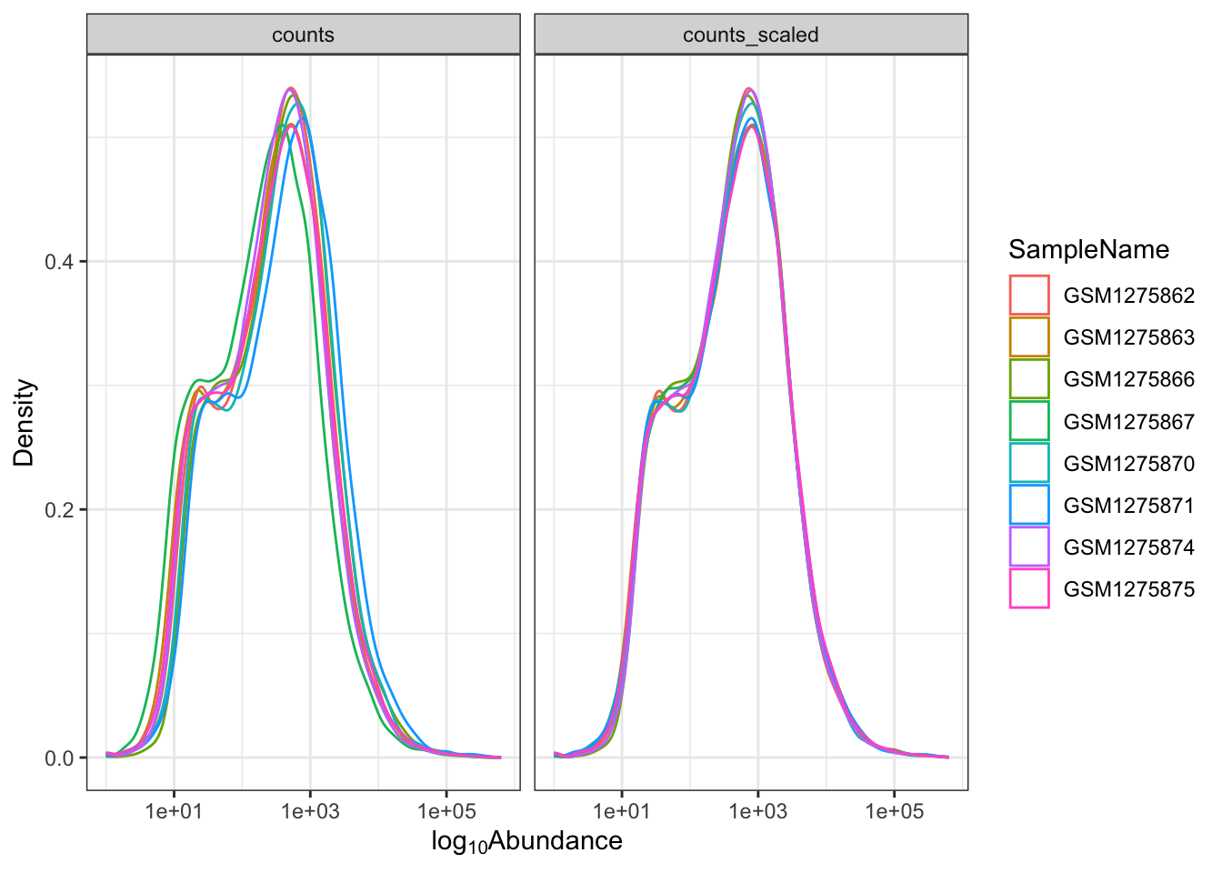
Let's see how this might work with our scaled_counts data. We want to plot both "counts" and "counts_scaled" together in a density plot to understand the distribution of the data. Did scaling the counts improve the distribution?
We can place "counts" and "counts_scaled" into a column named "source" and place their values in a column named "abundance".
#getting the data
scounts_long<- scaled_counts |>
  #pivot
  pivot_longer(cols = c("counts", "counts_scaled"),
               names_to = "source", values_to = "abundance")
#View
scounts_long |> select(source, abundance) |> head()
# A tibble: 6 × 2
  source        abundance
  <chr>             <dbl>
1 counts             679
2 counts_scaled      961.
3 counts             467
4 counts_scaled      661.
5 counts             260
6 counts_scaled      368.
Now let's create a density plot using ggplot2.
ggplot(data=scounts_long, aes(x = abundance + 1, color = SampleName))+
  geom_density() +
  facet_wrap(~source) +
  ggplot2::scale_x_log10() +
  theme_bw()+
  ylab("Density")+
  xlab(expression('log'[10]*'Abundance'))
Note
It's not important to understand the code here. This will make more sense in the next lesson.
Acknowledgements
Material from this lesson was either taken directly or adapted from the Intro to R and RStudio for Genomics lesson provided by datacarpentry.org and from a 2021 workshop entitled Introduction to Tidy Transciptomics by Maria Doyle and Stefano Mangiola. This lesson was also inspired by material from "Manipulating and analyzing data with dplyr", Introduction to data analysis with R and Bioconductor.