R Data Structures: Introducing Data Frames

Learning Objectives

1. Learn about data structures including factors, lists, data frames, and matrices.
2. Load, explore, and access data in a tabular format (data frames)
3. Learn to write out (export) data from the R environment

Data Structures

Data structures are objects that store data.

Previously, we learned that vectors are collections of values of the same type. A vector is also one of the most basic data structures.

Other common data structures in R include:

• factors
• lists
• data frames
• matrices

What are factors?

Factors are an important data structure in statistical computing. They are specialized vectors (ordered or unordered) for the storage of categorical data. While they appear to be character vectors, data in factors are stored as integers. These integers are associated with pre-defined levels, which represent the different groups or categories in the vector.

Important functions

• factor() - to create a factor and reorder levels
• as.factor() - to coerce to a factor
• levels() - view the levels of a factor
• nlevels() - return the number of levels

For example:

sex <- factor(c("M","F","F","M","M","M"))
levels(sex)

[1] "F" "M"

Check out the package forcats for managing and reordering factors.

Lists

Unlike an atomic vector, a list can contain multiple elements of different types, (e.g., character vector, numeric vector, list, data frame, matrix).

Important functions

• list() - create a list
• names() - create named elements (Also useful for vectors)
• lapply(), sapply() - for looping over elements of the list

Example

#Create a list
My_exp <- list(c("N052611", "N061011", "N080611", "N61311" ), 
               c("SRR1039508", "SRR1039509", "SRR1039512",
                 "SRR1039513", "SRR1039516", "SRR1039517",
                 "SRR1039520", "SRR1039521"),c(100,200,300,400))
#Look at the structure
str(My_exp)

List of 3
 $ : chr [1:4] "N052611" "N061011" "N080611" "N61311"
 $ : chr [1:8] "SRR1039508" "SRR1039509" "SRR1039512" "SRR1039513" ...
 $ : num [1:4] 100 200 300 400

#Name the elements of the list 
names(My_exp)<-c("cell_lines","sample_id","counts")
#See how the structure changes
str(My_exp)

List of 3
 $ cell_lines: chr [1:4] "N052611" "N061011" "N080611" "N61311"
 $ sample_id : chr [1:8] "SRR1039508" "SRR1039509" "SRR1039512" "SRR1039513" ...
 $ counts    : num [1:4] 100 200 300 400

#Subset the list
My_exp[[1]][2]

[1] "N061011"

My_exp$cell_lines[2]

[1] "N061011"

#Apply a function (remove the first index from each vector)
lapply(My_exp,function(x){x[-1]})

$cell_lines
[1] "N061011" "N080611" "N61311" 

$sample_id
[1] "SRR1039509" "SRR1039512" "SRR1039513" "SRR1039516" "SRR1039517"
[6] "SRR1039520" "SRR1039521"

$counts
[1] 200 300 400

We are not going to spend a lot of time on lists, but you should consider learning more about them in the future, as you may receive output at some point in the form of a list. For a brief introduction to lists, see the following resources:

• R4DS
• UVA list tutorial

Data Frames: Working with Tabular Data

In genomics, we work with a lot of tabular data - data organized in rows and columns. The data structure that stores this type of data is a data frame. Data frames are collections of vectors of the same length but can be of different types. Because we often have data of multiple types, it is natural to examine that data in a data frame.

You may be tempted to open and manually work with these data in excel. However, there are a number of reasons why this can be to your detriment. First, it is very easy to make mistakes when working with large amounts of tabular data in excel. Have you ever mistakenly left out a column or row while sorting data? Second, many of the files that we work with are so large (big data) that excel and your local machine do not have the bandwidth to handle them. Third, you will likely need to apply analyses that are unavailable in excel. Lastly, it is difficult to keep track of any data manipulation steps or analyses in a point and click environment like excel.

R, on the other hand, can make analyzing tabular data more efficient and reproducible. But before getting into working with this data in R, let's review some best practices for data management.

Best Practices for organizing genomic data

1. "Keep raw data separate from analyzed data" -- datacarpentry.org

   For large genomic data sets, you may want to include a project folder with two main subdirectories (i.e., raw_data and data_analysis). You may even consider changing the permissions (check out the unix command chmod) in your raw directory to make those files read only. Keeping raw data separate is not a problem in R, as one must explicitly import and export data.

2. "Keep spreadsheet data Tidy" -- datacarpentry.org

   Data organization can be frustrating, and many scientists devote a great deal of time and energy toward this task. Keeping data tidy, which we will talk about more next lesson, can make data science more efficient, effective, and reproducible.

3. "Trust but verify" -- datacarpentry.org

   R makes data analysis more reproducible and can eliminate some mistakes from human error. However, you should approach data analysis with a plan, and make sure you understand what a function is doing before applying it to your data. Hopefully, today's lesson will help with this. Often using small subsets of data can be used as a form of data debugging to make sure the expected result materialized.

   Some functions for creating practice data include: data.frame(), rep(), seq(), rnorm(), sample() and others. See some examples here.

Introducing the airway data

There are data sets available in R to practice with or showcase different packages. For today's lesson and the remainder of this course, we will use data from the Bioconductor package airway to showcase tools used for data wrangling and visualization. The use of this data was inspired by a 2021 workshop entitled Introduction to Tidy Transciptomics by Maria Doyle and Stefano Mangiola. Code has been adapted from this workshop to explore tidyverse functionality.

The airway data is from Himes et al. (2014). These data, which are contained within a RangedSummarizedExperiment, object are from a bulk RNAseq experiment. In the experiment, the authors "characterized transcriptomic changes in four primary human ASM cell lines that were treated with dexamethasone," a common therapy for asthma. The airway package includes RNAseq count data from 8 airway smooth muscle cell samples. Each cell line includes a treated and untreated negative control.

Do not worry about the RangedSummarizedExperiment. The data we will use today and next week have been provided to you in the following files:

• filtlowabund_scaledcounts_airways.txt - Includes scaled transcript count data.
• diffexp_results_edger_airways.txt - Includes results from differential expression analysis using EdgeR.

Object (.rds) files have also been included.

Importing / exporting data

Before we can do anything with our data, we need to first import it into R. There are several ways to do this.

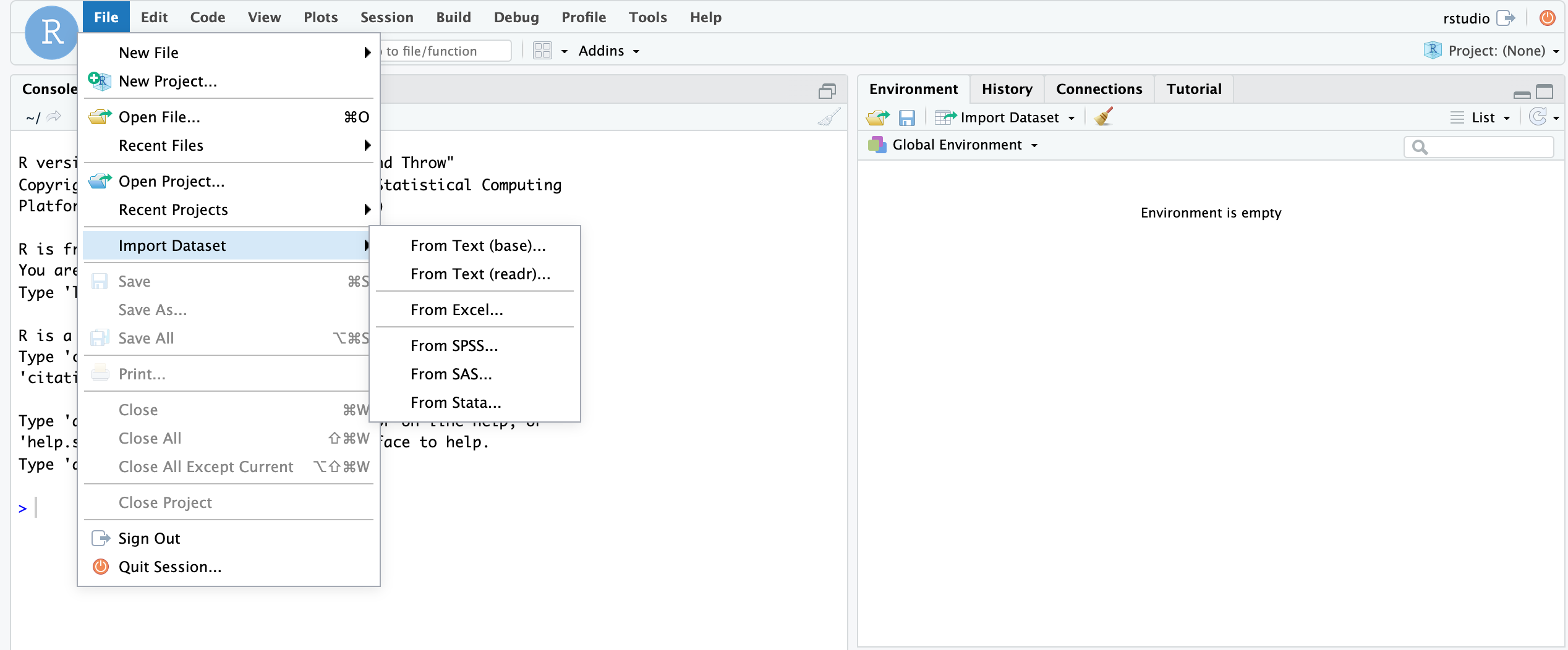
First, the RStudio IDE has a dropdown menu for data import. Simply go to File > Import Dataset and select one of the options and follow the prompts.

Let's focus on the base R import functions. These include read.csv(), read.table(), read.delim(), etc. You should examine the function arguments (e.g., ?read.delim()) to get an idea of what is happening at import and ensure that your data is being parsed correctly.

#Let's import our data and save to an object called scaled_counts
scaled_counts<-read.delim(
  "./data/filtlowabund_scaledcounts_airways.txt", as.is=TRUE)

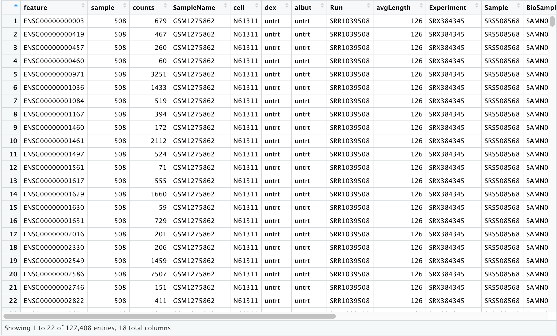
We can now see this object in our RStudio environment pane.

This object can be viewed by clicking on it in the environment pane. Alternatively, you can use View(scaled_counts).

To import an existing object, we usereadRDS().

#Let's import our data from the .rds file
#and save to an object called scaled_counts_rds
scaled_counts_rds<-
  data.frame(readRDS("./data/filtlowabund_scaledcounts_airways.rds"))

To export data to file, you will use similar functions (write.table(),write.csv(),saveRDS(), etc.). We will show how these work later in the lesson.

Examining and summarizing data frames

The object that we imported, scaled_counts, is a data frame. Let's learn a bit more about our data frame. First, we can learn more about the structure of our data using str(). We have seen this function in use previously.

str(scaled_counts)

'data.frame':   127408 obs. of  18 variables:
 $ feature      : chr  "ENSG00000000003" "ENSG00000000419" "ENSG00000000457" "ENSG00000000460" ...
 $ sample       : int  508 508 508 508 508 508 508 508 508 508 ...
 $ counts       : int  679 467 260 60 3251 1433 519 394 172 2112 ...
 $ SampleName   : chr  "GSM1275862" "GSM1275862" "GSM1275862" "GSM1275862" ...
 $ cell         : chr  "N61311" "N61311" "N61311" "N61311" ...
 $ dex          : chr  "untrt" "untrt" "untrt" "untrt" ...
 $ albut        : chr  "untrt" "untrt" "untrt" "untrt" ...
 $ Run          : chr  "SRR1039508" "SRR1039508" "SRR1039508" "SRR1039508" ...
 $ avgLength    : int  126 126 126 126 126 126 126 126 126 126 ...
 $ Experiment   : chr  "SRX384345" "SRX384345" "SRX384345" "SRX384345" ...
 $ Sample       : chr  "SRS508568" "SRS508568" "SRS508568" "SRS508568" ...
 $ BioSample    : chr  "SAMN02422669" "SAMN02422669" "SAMN02422669" "SAMN02422669" ...
 $ transcript   : chr  "TSPAN6" "DPM1" "SCYL3" "C1orf112" ...
 $ ref_genome   : chr  "hg38" "hg38" "hg38" "hg38" ...
 $ .abundant    : logi  TRUE TRUE TRUE TRUE TRUE TRUE ...
 $ TMM          : num  1.06 1.06 1.06 1.06 1.06 ...
 $ multiplier   : num  1.42 1.42 1.42 1.42 1.42 ...
 $ counts_scaled: num  960.9 660.9 367.9 84.9 4600.7 ...

str() shows us that we are looking at a data frame object with 127,408 observations in 18 variables (or columns). The column names are to the far left preceded by a $. This is a data frame accessor, and we will see how this works later. We can also see the data type (character, integer, logical, numeric) after the column name. This will help us understand how we can transform and visualize the data in these columns.

We can also get an overview of summary statistics of this data frame using summary().

summary(scaled_counts)

   feature              sample          counts        SampleName       
 Length:127408      Min.   :508.0   Min.   :     0   Length:127408     
 Class :character   1st Qu.:511.2   1st Qu.:    66   Class :character  
 Mode  :character   Median :514.5   Median :   310   Mode  :character  
                    Mean   :514.5   Mean   :  1376                     
                    3rd Qu.:517.8   3rd Qu.:   960                     
                    Max.   :521.0   Max.   :513766                     
     cell               dex               albut               Run           
 Length:127408      Length:127408      Length:127408      Length:127408     
 Class :character   Class :character   Class :character   Class :character  
 Mode  :character   Mode  :character   Mode  :character   Mode  :character  



   avgLength      Experiment           Sample           BioSample        
 Min.   : 87.0   Length:127408      Length:127408      Length:127408     
 1st Qu.:100.2   Class :character   Class :character   Class :character  
 Median :123.0   Mode  :character   Mode  :character   Mode  :character  
 Mean   :113.8                                                           
 3rd Qu.:126.0                                                           
 Max.   :126.0                                                           
  transcript         ref_genome        .abundant           TMM        
 Length:127408      Length:127408      Mode:logical   Min.   :0.9512  
 Class :character   Class :character   TRUE:127408    1st Qu.:0.9706  
 Mode  :character   Mode  :character                  Median :1.0052  
                                                      Mean   :1.0006  
                                                      3rd Qu.:1.0257  
                                                      Max.   :1.0553  
   multiplier    counts_scaled     
 Min.   :1.026   Min.   :     0.0  
 1st Qu.:1.230   1st Qu.:    95.4  
 Median :1.467   Median :   445.8  
 Mean   :1.466   Mean   :  1933.7  
 3rd Qu.:1.581   3rd Qu.:  1369.6  
 Max.   :2.136   Max.   :632885.3  

Our data frame has 18 variables, so we get 18 fields that summarize the data. Counts, avgLength, TMM, multiplier, and counts_scaled are numerical data and so we get summary statistics on the min and max values for these columns, as well as mean, median, and interquartile ranges.

What is the length of our data.frame? What are the dimensions?

#length returns the number of columns
length(scaled_counts)

[1] 18

#dimensions, returns the row and column numbers
dim(scaled_counts)  

[1] 127408     18

Other useful functions for inspecting data frames

Size:
nrow() - number of rows
ncol() - number of columns

Content:
head() - returns first 6 rows by default
tail() - returns last 6 rows by default

Names:
colnames() - returns column names
rownames() - returns row names

Section content from "Starting with Data", Introduction to data analysis with R and Bioconductor.

Data frame coercion and accessors

Notice that "sample" was treated as numeric, rather than as a character vector. If we intend to work with this column, we will need to convert it or coerce it to a character or factor vector.

We can access a column of our data frame using [], [[]], or using the $. These behave slightly differently, as we will see.

Let's access "sample" from scaled_counts. We use head() to limit the printed output.

#Using $
head(scaled_counts$sample)  

[1] 508 508 508 508 508 508

#Using []  
head(scaled_counts["sample"])

  sample
1    508
2    508
3    508
4    508
5    508
6    508

#Using [[]]  
head(scaled_counts[["sample"]])

[1] 508 508 508 508 508 508

Let's convert the "sample" column from an integer to a character vector. This is known as coercion.

#We can see that sample is being treated as numeric
is.numeric(scaled_counts$sample) 

[1] TRUE

#let's convert it to a character vector
scaled_counts$sample<-as.character(scaled_counts$sample)
#check this
is.character(scaled_counts$sample) 

[1] TRUE

#check this
is.numeric(scaled_counts$sample) 

[1] FALSE

See other related functions (e.g., as.factor(),as.numeric()).

Be careful with data coercion. What happens if we change a character vector into a numeric?

#A warning is thrown and the entire column is filled with NA
head(as.numeric(scaled_counts$Sample)) 

Warning in head(as.numeric(scaled_counts$Sample)): NAs introduced by coercion

[1] NA NA NA NA NA NA

Some helpful things to remember

• When you explicitly coerce one data type into another (this is known as explicit coercion), be careful to check the result. Ideally, you should try to see if its possible to avoid steps in your analysis that force you to coerce.
• R will sometimes coerce without you asking for it. This is called (appropriately) implicit coercion. For example when we tried to create a vector with multiple data types, R chose one type through implicit coercion.
• Check the structure (str()) of your data frames before working with them! ---datacarpentry.org

Using colnames() to rename columns

colnames() will return a vector of column names from our data frame. We can use this vector and [] subsetting to easily modify column names.

For example, let's rename the column "Sample" to "Accession".

#Let's rename "Sample" to "Accession"
colnames(scaled_counts)[11]<-"Accession" 

#if unsure of the index of the "Sample" column, you could use which()
which(colnames(scaled_counts)=="Sample") 

#or you could get the indices in a data frame
data.frame(colnames(scaled_counts))


#or something like this
colnames(scaled_counts)[colnames(scaled_counts) == 
                          "Sample"] <- "Accession"

Test your learning

Which of the following will NOT print the "Run" column from scaled_counts?
a. scaled_counts$Run
b. scaled_counts["Run"]
c. scaled_counts[8,]
d. scaled_counts[8]

What is the column index for "avgLength" from the scaled_counts df?
a. 3
b. 8
c. 12
d. 9

Exporting Data (Save the data frame to a file)

If we want to export our df (scaled_counts) to use with another program, we can write out to a file.

write.table(scaled_counts, 
            file = "scaled_counts_mod.txt",
            quote=FALSE,row.names=FALSE,sep="\t") 

If you are unsure what these arguments mean, use ?write.table().

Data Matrices

Another important data structure in R is the data matrix. Data frames and data matrices are similar in that both are tabular in nature and are defined by dimensions (i.e., rows (m) and columns (n), commonly denoted m x n). However, a matrix contains only values of a single type (i.e., numeric, character, logical, etc.).

Elements in a matrix and a data frame can be referenced by using their row and column indices (for example, a[1,1] references the element in row 1 and column 1).

Below, we create the object a1, a 3 row by 4 column matrix.

a1 <- matrix(c(3,4,2,4,6,3,8,1,7,5,3,2), ncol=4)
a1

     [,1] [,2] [,3] [,4]
[1,]    3    4    8    5
[2,]    4    6    1    3
[3,]    2    3    7    2

Using the typeof() and class() command, we see that the elements in a1 are double and a1 a matrix, respectively.

typeof(a1)

[1] "double"

class(a1)

[1] "matrix" "array" 

Earlier, we mentioned that elements in a matrix can be referenced by their row and column number. Below, we extract the element in the 3rd row and 4th column of a1 (which is 2)

a1[3,4] ## returns 2

[1] 2

We can assign column and row names to a matrix.

colnames(a1) <- c("control1","control2","tumor1","tumor2")
rownames(a1) <- c("ADA","AMPD2","HPRT")
a1

      control1 control2 tumor1 tumor2
ADA          3        4      8      5
AMPD2        4        6      1      3
HPRT         2        3      7      2

But, we cannot reference columns using $.

a1$control1

Error in a1$control1: $ operator is invalid for atomic vectors

We can create matrices mixed with words and numbers (see a2).

a2 <- matrix(c("apples","pears","oranges",50,25,75), ncol=2)
a2

     [,1]      [,2]
[1,] "apples"  "50"
[2,] "pears"   "25"
[3,] "oranges" "75"

But, R will coerce all of the elements to the same type, in this case character.

typeof(a2)

[1] "character"

typeof(a2[,2])

[1] "character"

class(a2)

[1] "matrix" "array" 

We can also perform mathematical operations on matrices.

a3 <- 5
a3

[1] 5

Below we multiply every element in a1 by a3 and store in a4. Note, we are still left with a 3 by 4 matrix except the values have been multiplied by the value assigned to a3 (5).

a4 <- a1*a3
a1

      control1 control2 tumor1 tumor2
ADA          3        4      8      5
AMPD2        4        6      1      3
HPRT         2        3      7      2

a4

      control1 control2 tumor1 tumor2
ADA         15       20     40     25
AMPD2       20       30      5     15
HPRT        10       15     35     10

Here are some similarities and differences between matrices and data frames:

                             Characteristic Matrix Data.frame
1                 is rectangular data table    yes        yes
2               can perform math operations    yes        yes
3                needs homogenous data type    yes         no
4          can have heterogeneous data type     no        yes
5 can reference using row and column number    yes        yes
6              can reference column using $     no        yes
7                      can use for plotting    yes        yes

Acknowledgements

Material from this lesson was either taken directly or adapted from Intro to R and RStudio for Genomics provided by datacarpentry.org and from a 2021 workshop entitled Introduction to Tidy Transciptomics by Maria Doyle and Stefano Mangiola.

Resources

1. BaseR cheatsheet