Lesson 7: Quantifying Gene Expression
Lesson 6 Review
Lesson 6 introduced alignment of bulk RNA sequences in order to find where in the genome each read came from. Post alignment QC metrics were also covered. The next step, covered in this class will deal with quantifying gene expression based on the number of reads that map to each gene.
Learning objectives
After this lesson, participants will be able to:
- Describe the goal of gene expression quantification in bulk RNA sequencing and name tools that can be used for this task.
- Understand the content of GTF annotation file and why it is needed in quantification.
- Interpret post quantification QC metrics.
- Become familiar with the quantification table.
Goals for Gene Expression Quantification in Bulk RNA Sequencing
When the origin in the genome of each sequencing read in bulk RNA has been identified, the next step is quantifying gene expression levels. Here, the number of reads that map to a particular gene or transcript is used as an estimate for its expression level. This should be a simple counting exercise but the process is more complicated.
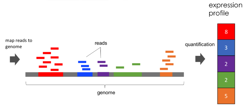
Image was modified from https://mbernste.github.io/posts/rna_seq_basics/
As it turns out, there are various scenarios in the gene expression quantification process. For instance:
- Reads that map to multiple genes.
- Reads that partially overlap a gene.
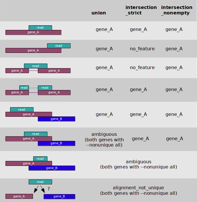 Image source: https://htseq.readthedocs.io/en/latest/htseqcount.html
Tools used for bulk RNA sequencing expression quantification include HTSeq, featureCounts, and RSEM. Below is a comparison of these three tools. RSEM is more sophisticated and can better quantify reads that map to multiple spots in the genome so it is used in RENEE.
| HTSeq | featureCounts | RSEM |
|---|---|---|
| Overlap based | Overlap based | Expectation-Maximization |
| Assign fraction to multi-mappers | Assign fraction to multi-mappers | More accurately quantify expression for multi-mappers |
| No long reads | Long reads | Long reads |
Pseudo aligners such as Salmon can map and quantify to transcriptome at the same time.
Annotation Files
During the alignment step, a reference genome or transcriptome is needed. This is to guide the aligner as it determines where is the best match for each read. When it comes to quantifying expression, a file that contains information on the location of genes, transcripts, exons, coding sequences, introns is needed. A common format is the General Transfer Format (GTF), which is tab separated table that holds genomic annotations. Below is a glimpse of the contents of a GTF file.
| Chromosome | Annotation source | Feature | Start | End | Score | Strand | Frame | Attributes |
|---|---|---|---|---|---|---|---|---|
| chr22 | ENSEMBL | gene | 10736171 | 10736283 | . | - | . | **"gene_id ""ENSG00000277248.1""; gene_type ""snRNA""; gene_status ""NOVEL""; gene_name ""U2""; level 3;"** |
| chr22 | ENSEMBL | transcript | 10736171 | 10736283 | . | - | . | **"gene_id ""ENSG00000277248.1""; transcript_id ""ENST00000615943.1""; gene_type ""snRNA""; gene_status ""NOVEL""; gene_name ""U2""; transcript_type ""snRNA""; transcript_status ""NOVEL""; transcript_name ""U2.14-201""; level 3; tag ""basic""; transcript_support_level ""NA"";"** |
| chr22 | ENSEMBL | exon | 10736171 | 10736283 | . | - | . | **"gene_id ""ENSG00000277248.1""; transcript_id ""ENST00000615943.1""; gene_type ""snRNA""; gene_status ""NOVEL""; gene_name ""U2""; transcript_type ""snRNA""; transcript_status ""NOVEL""; transcript_name ""U2.14-201""; exon_number 1; exon_id ""ENSE00003736336.1""; level 3; tag ""basic""; transcript_support_level ""NA"";"** |
| chr22 | ENSEMBL | gene | 10936023 | 10936161 | . | - | . | **"gene_id ""ENSG00000274237.1""; gene_type ""miRNA""; gene_status ""NOVEL""; gene_name ""CU459211.1""; level 3;"** |
| chr22 | ENSEMBL | transcript | 10936023 | 10936161 | . | - | . | **"gene_id ""ENSG00000274237.1""; transcript_id ""ENST00000618365.1""; gene_type ""miRNA""; gene_status ""NOVEL""; gene_name ""CU459211.1""; transcript_type ""miRNA""; transcript_status ""NOVEL""; transcript_name ""CU459211.1-201""; level 3; tag ""basic""; transcript_support_level ""NA"";"** |
| chr22 | ENSEMBL | exon | 10936023 | 10936161 | . | - | . | **"gene_id ""ENSG00000274237.1""; transcript_id ""ENST00000618365.1""; gene_type ""miRNA""; gene_status ""NOVEL""; gene_name ""CU459211.1""; transcript_type ""miRNA""; transcript_status ""NOVEL""; transcript_name ""CU459211.1-201""; exon_number 1; exon_id ""ENSE00003712615.1""; level 3; tag ""basic""; transcript_support_level ""NA"";"** |
| chr22 | ENSEMBL | gene | 11065974 | 11067346 | . | - | . | **"gene_id ""ENSG00000280363.1""; gene_type ""protein_coding""; gene_status ""KNOWN""; gene_name ""CU104787.1""; level 3;"** |
| chr22 | ENSEMBL | transcript | 11065974 | 11067346 | . | - | . | **"gene_id ""ENSG00000280363.1""; transcript_id ""ENST00000623473.1""; gene_type ""protein_coding""; gene_status ""KNOWN""; gene_name ""CU104787.1""; transcript_type ""protein_coding""; transcript_status ""KNOWN""; transcript_name ""CU104787.1-201""; level 3; protein_id ""ENSP00000485388.1""; tag ""basic""; transcript_support_level ""5""; tag ""appris_principal_1"";"** |
| chr22 | ENSEMBL | exon | 11065974 | 11066015 | . | - | . | **"gene_id ""ENSG00000280363.1""; transcript_id ""ENST00000623473.1""; gene_type ""protein_coding""; gene_status ""KNOWN""; gene_name ""CU104787.1""; transcript_type ""protein_coding""; transcript_status ""KNOWN""; transcript_name ""CU104787.1-201""; exon_number 2; exon_id ""ENSE00003755067.1""; level 3; protein_id ""ENSP00000485388.1""; tag ""basic""; transcript_support_level ""5""; tag ""appris_principal_1"";"** |
| chr22 | ENSEMBL | CDS | 11065974 | 11066015 | . | - | 0 | **"gene_id ""ENSG00000280363.1""; transcript_id ""ENST00000623473.1""; gene_type ""protein_coding""; gene_status ""KNOWN""; gene_name ""CU104787.1""; transcript_type ""protein_coding""; transcript_status ""KNOWN""; transcript_name ""CU104787.1-201""; exon_number 2; exon_id ""ENSE00003755067.1""; level 3; protein_id ""ENSP00000485388.1""; tag ""basic""; transcript_support_level ""5""; tag ""appris_principal_1"";"** |
| chr22 | ENSEMBL | gene | 11066501 | 11068089 | . | + | . | **"gene_id ""ENSG00000279973.1""; gene_type ""protein_coding""; gene_status ""KNOWN""; gene_name ""BAGE5""; level 3;"** |
| chr22 | ENSEMBL | transcript | 11066501 | 11068089 | . | + | . | **"gene_id ""ENSG00000279973.1""; transcript_id ""ENST00000624155.1""; gene_type ""protein_coding""; gene_status ""KNOWN""; gene_name ""BAGE5""; transcript_type ""protein_coding""; transcript_status ""KNOWN""; transcript_name ""BAGE5-201""; level 3; protein_id ""ENSP00000485185.1""; tag ""basic""; transcript_support_level ""1""; tag ""appris_principal_1"";"** |
| chr22 | ENSEMBL | exon | 11066501 | 11066515 | . | + | . | **"gene_id ""ENSG00000279973.1""; transcript_id ""ENST00000624155.1""; gene_type ""protein_coding""; gene_status ""KNOWN""; gene_name ""BAGE5""; transcript_type ""protein_coding""; transcript_status ""KNOWN""; transcript_name ""BAGE5-201""; exon_number 1; exon_id ""ENSE00003758096.1""; level 3; protein_id ""ENSP00000485185.1""; tag ""basic""; transcript_support_level ""1""; tag ""appris_principal_1"";"** |
Quantification Output
RENEE saves the expression results in the DEG_ALL folder of the output directory. Change into it and list the contents one item per line.
cd DEG_ALL
ls -1
RSEM provides quantification estimates on the gene and isoform level. Per sample basis (sample.RSEM.genes.results and sample.RSEM.isoforms.results) as well as combined quantifications for all samples (see RSEM.genes.expected_count.all_samples.txt and RSEM.isoforms.expected_count.all_samples.txt) are provided. The files labeled FPKM and TPM are normalized expression estimates, however differential expression tools such as DESeq2 and edgeR do not use these as they take unormalized expression data as input. For the purposes of the class, look at RSEM.genes.expected_count.all_samples.txt.
-rw-r----- 1 $USER $USER  49351 Jul  3 16:38 combined_TIN.tsv
-rw-r----- 1 $USER $USER 274485 Jul  3 16:38 hcc1395_normal_rep1.RSEM.genes.results
-rw-r----- 1 $USER $USER 809683 Jul  3 16:38 hcc1395_normal_rep1.RSEM.isoforms.results
drwxr-x--- 2 $USER $USER   4096 Jul  3 16:38 hcc1395_normal_rep1.RSEM.stat
-rw-r----- 1 $USER $USER     98 Jul  3 16:38 hcc1395_normal_rep1.RSEM.time
-rw-r----- 1 $USER $USER 274483 Jul  3 16:38 hcc1395_normal_rep2.RSEM.genes.results
-rw-r----- 1 $USER $USER 809538 Jul  3 16:38 hcc1395_normal_rep2.RSEM.isoforms.results
drwxr-x--- 2 $USER $USER   4096 Jul  3 16:38 hcc1395_normal_rep2.RSEM.stat
-rw-r----- 1 $USER $USER     98 Jul  3 16:38 hcc1395_normal_rep2.RSEM.time
-rw-r----- 1 $USER $USER 274467 Jul  3 16:38 hcc1395_normal_rep3.RSEM.genes.results
-rw-r----- 1 $USER $USER 809708 Jul  3 16:38 hcc1395_normal_rep3.RSEM.isoforms.results
drwxr-x--- 2 $USER $USER   4096 Jul  3 16:38 hcc1395_normal_rep3.RSEM.stat
-rw-r----- 1 $USER $USER     98 Jul  3 16:38 hcc1395_normal_rep3.RSEM.time
-rw-r----- 1 $USER $USER 274554 Jul  3 16:38 hcc1395_tumor_rep1.RSEM.genes.results
-rw-r----- 1 $USER $USER 809469 Jul  3 16:38 hcc1395_tumor_rep1.RSEM.isoforms.results
drwxr-x--- 2 $USER $USER   4096 Jul  3 16:38 hcc1395_tumor_rep1.RSEM.stat
-rw-r----- 1 $USER $USER     98 Jul  3 16:38 hcc1395_tumor_rep1.RSEM.time
-rw-r----- 1 $USER $USER 274594 Jul  3 16:38 hcc1395_tumor_rep2.RSEM.genes.results
-rw-r----- 1 $USER $USER 809729 Jul  3 16:38 hcc1395_tumor_rep2.RSEM.isoforms.results
drwxr-x--- 2 $USER $USER   4096 Jul  3 16:38 hcc1395_tumor_rep2.RSEM.stat
-rw-r----- 1 $USER $USER     98 Jul  3 16:38 hcc1395_tumor_rep2.RSEM.time
-rw-r----- 1 $USER $USER 274547 Jul  3 16:38 hcc1395_tumor_rep3.RSEM.genes.results
-rw-r----- 1 $USER $USER 809614 Jul  3 16:38 hcc1395_tumor_rep3.RSEM.isoforms.results
drwxr-x--- 2 $USER $USER   4096 Jul  3 16:38 hcc1395_tumor_rep3.RSEM.stat
-rw-r----- 1 $USER $USER     98 Jul  3 16:38 hcc1395_tumor_rep3.RSEM.time
-rw-r----- 1 $USER $USER  81819 Jul  3 16:38 RSEM.genes.expected_count.all_samples.txt
-rw-r----- 1 $USER $USER  77987 Jul  3 16:38 RSEM.genes.expected_counts.all_samples.matrix
-rw-r----- 1 $USER $USER  81809 Jul  3 16:38 RSEM.genes.expected_counts.all_samples.reformatted.tsv
-rw-r----- 1 $USER $USER  85394 Jul  3 16:38 RSEM.genes.FPKM.all_samples.txt
-rw-r----- 1 $USER $USER  86000 Jul  3 16:38 RSEM.genes.TPM.all_samples.txt
-rw-r----- 1 $USER $USER 386203 Jul  3 16:38 RSEM.isoforms.expected_count.all_samples.txt
-rw-r----- 1 $USER $USER 277331 Jul  3 16:38 RSEM.isoforms.expected_counts.all_samples.matrix
-rw-r----- 1 $USER $USER 392811 Jul  3 16:38 RSEM.isoforms.FPKM.all_samples.txt
-rw-r----- 1 $USER $USER 394765 Jul  3 16:38 RSEM.isoforms.TPM.all_samples.txt
Use the column command construct below to get a glimpse of the gene level expression estimates for all samples saved in RSEM.genes.expected_count.all_samples.txt.
columnis a command that prints tabular data to the terminal with columns nicely aligned.-tis an option to tellcolumnto create a table.- The argument is the file that the user wants to display (ie.
RSEM.genes.expected_count.all_samples.txt).
- The output of
columnis sent tolessusing pipe (|). The-Soption inlessenables horizontal scrolling on the terminal.
column -t RSEM.genes.expected_count.all_samples.txt | less -S
gene_id             GeneName           hcc1395_normal_rep1  hcc1395_normal_rep2  hcc1395_normal_rep3  hcc1395_tumor_rep1  hcc1395_tumor_rep2  hcc1395_tumor_rep3
ENSG00000276871.1   5_8S_rRNA          0.0                  0.0                  0.0                  0.0                 0.0                 0.0
ENSG00000128274.17  A4GALT             187.0                212.0                212.0                266.0               240.0               255.0
ENSG00000225293.1   ABCD1P4            0.0                  0.0                  0.0                  0.0                 0.0                 0.0
ENSG00000229107.2   ABHD17AP4          5.0                  14.0                 4.0                  9.0                 12.0                5.82
ENSG00000263366.2   ABHD17AP5          0.0                  0.0                  2.0                  0.0                 0.0                 1.18
ENSG00000100412.17  ACO2               3538.0               3517.89              3508.76              2181.0              2315.0              2316.0
Quantification Metrics
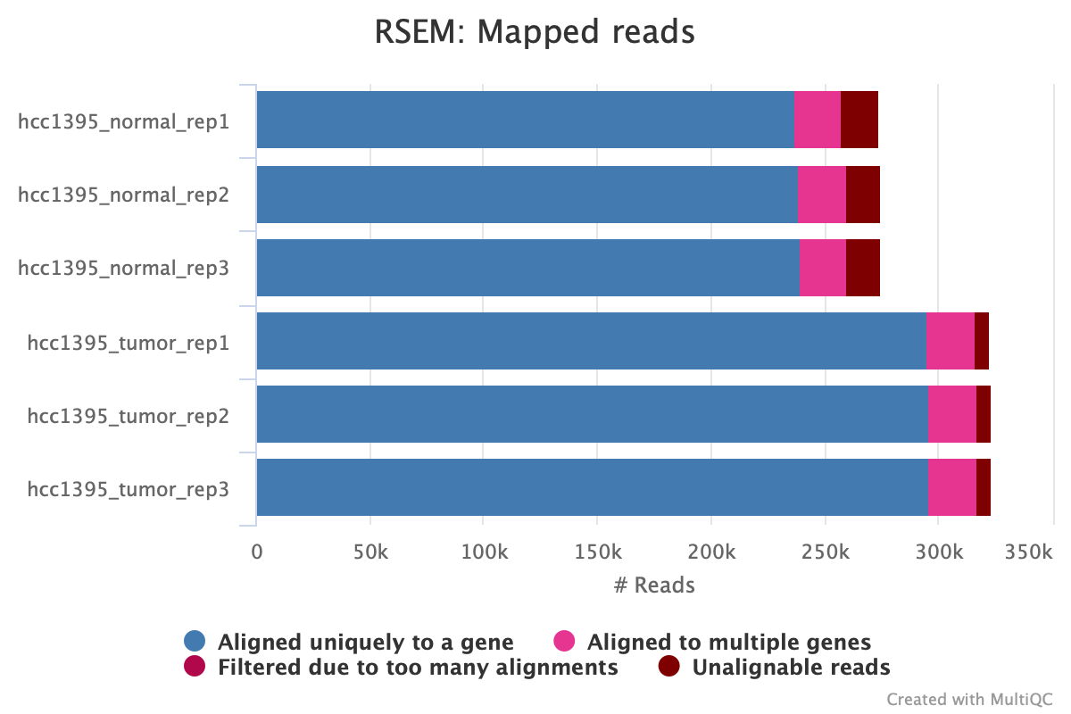
An important metric for estimation of gene expression is how many reads was the quantifier able to assign to a gene or transcript. Below is a plot that shows this for RSEM. For normal samples, approximately 87% of aligned reads were assigned to a unique gene, while tumor samples had approximately a 91% assignment rate.
Gene Coverage
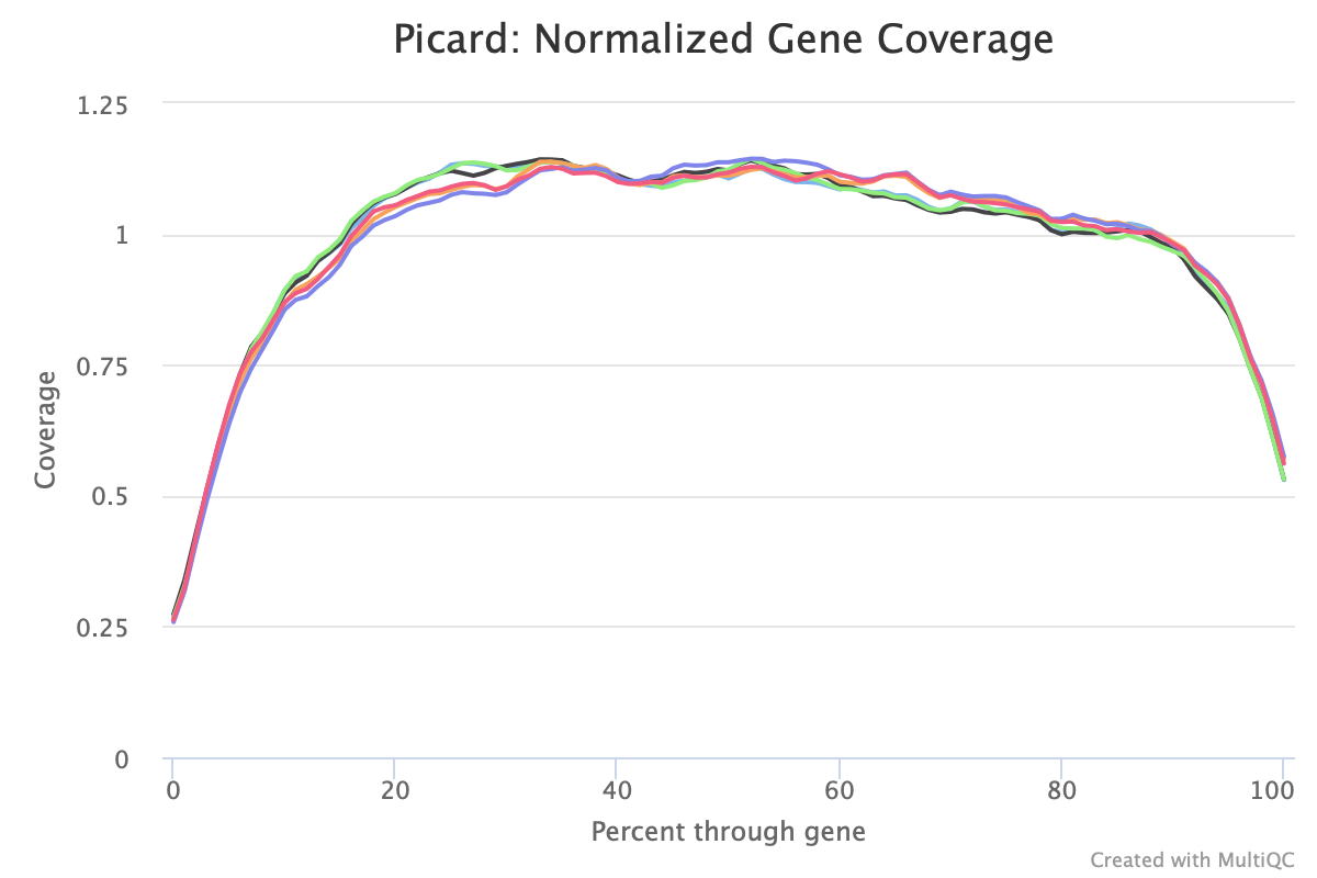
Picard’s normalized gene-body coverage plot shows how sequencing coverage is distributed from the annotated 5′ end to the 3′ end of transcripts. It is mainly used to detect technical coverage bias, such as RNA degradation, incomplete reverse transcription, or library-preparation bias.
- The samples have very similar profiles, which suggests good consistency.
- Coverage is relatively flat across most of the gene body.
- The lower coverage at both ends is common and can result from transcript-end annotation, read-length constraints, fragmentation, and alignment effects. There is no strong 3′ or 5′ bias visible.
Transcript Integrity
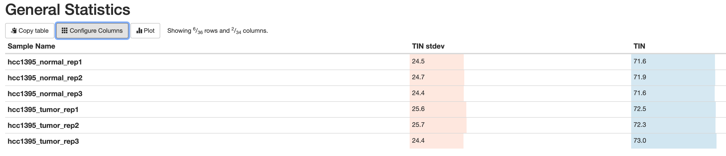
RSeQC calculates a transcript integrity number (TIN) that informs of the intactness of RNA at the transcript level and acts as metric for determining whether there is uniform read coverage across the transcript. This can be reviewed in the general statistics table. Just select "Configure Columns" and deselect everything except "RSeQC TIN stdev" and "RSeQC TIN". The fact that all TIN in this study are greater than 70% means that there is no degradation and uniform read coverage across the transcript. The high standard deviation could be due to low expression genes no have uniform coverage or certain transcripts just produce non-uniform coverage.
RNA Report
The file RNA_Report.html in the Reports directory of the output folder provides additional QC metrics for the RNA sequencing study. This report provides a metadata table provides information including total number of read pairs in a sample, GC percentage, average mapping quality, coverage, median TIN, and flow cell in which the sample was sequenced on.

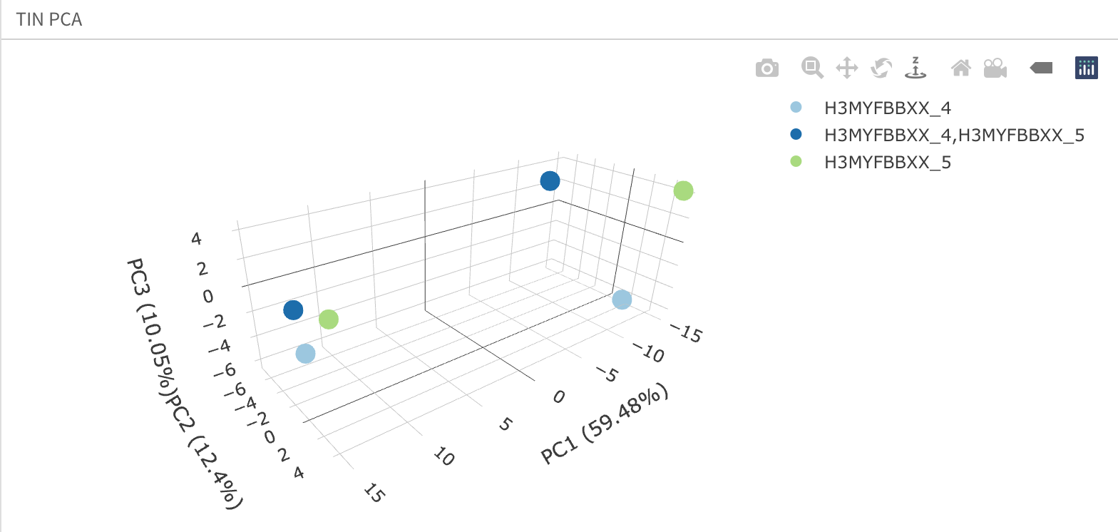
Below this table are two Principle Components (PCA) plots. One of which shows whether flow cell lane (legend) influences transcript integrity or TIN. In this case, TIN is not influenced by flow cell lane as we can distinguished clusters of samples from each flow cell clustering together and segregated along PC1 from the other trio. Mousing over this interactive plot, users will learn that in terms of TIN, tumor samples are clustered together and have similar TIN as do the normal samples. If flow cell affected TIN, then it would be expected that dots of the same color will cluster together more closely.
Moving to the subplots tab users will see 2 dimensional PCA plots indicating how differing QC metrics influence expression. As PC1 accounts for greater than 80% of the variance in these PCA plots, it can be concluded that it is expression that is driving apart the samples in the two clusters while QC metrics such as median TIN (medTIN) and flow cell lane play a minor role in differentiating between samples.

