Lesson 1: What Is Differential Expression Analysis?
Learning Objectives
By the end of this lesson, learners should be able to:
- identify the RNA-Seq count matrix and understand the data within;
- explain what differential expression analysis tests in an RNA-Seq experiment;
- describe why raw read counts and absolute abundances are not directly comparable across samples;
- distinguish common normalization strategies and when they are appropriate;
- identify common warning signs from QC that should be addressed before DEG testing;
- name the most widely used DE tools and know where to find them.
- know where to look when a specialized experimental design calls for a method beyond DESeq2, edgeR, or limma;
- know where to go next, iDEP for a GUI-driven analysis, or R/Python for full flexibility.
1. What Can We Do with a Count Matrix?
We are at the point in our workflow where we have a count matrix and sample metadata. The count matrix is the hub of our analysis. From it, we can do quality control (QC), filtering, differential expression (DE) testing, and pathway interpretation.
Where is my count matrix?
The RENEE workflow outputs multiple count matrices to DEG_ALL. This directory contains multiple count matrices by sample, across all samples, and by gene or isoform. See the RENEE documentation for details.
For this lesson, we will focus on the gene level counts across all samples. These are found in RSEM.genes.expected_count.all_samples.txt. If you do not have this file, you can copy or download it from /data/classes/BTEP/hcc1395_renee_out/DEG_ALL. We will discuss how to access this file for iDEP at the end of this lesson.
The count matrix is usually a tab-delimited text file with rows as genes and columns as samples. The first column is usually gene identifiers, and the first row is usually sample identifiers.
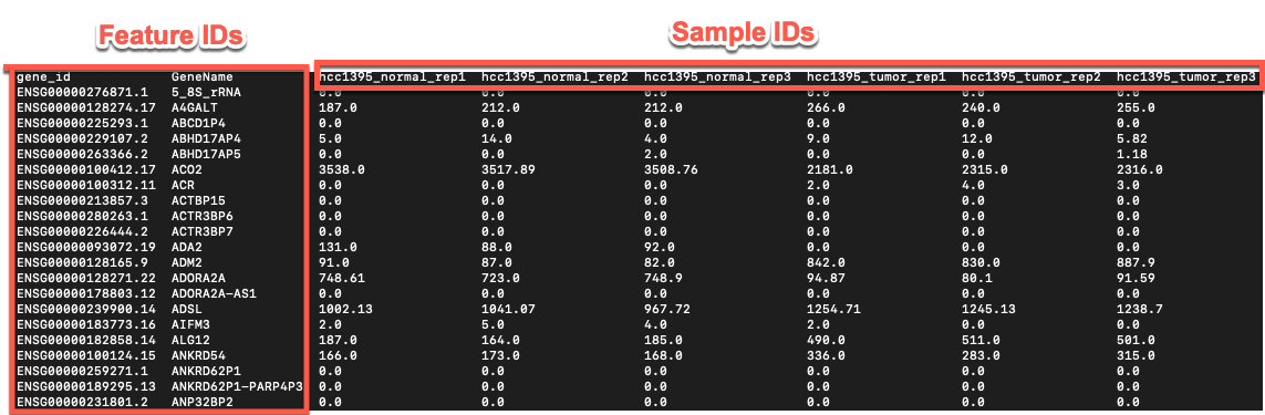
Figure 1: Gene Level Count Matrix from RENEE (ALL Samples)
2. The Core Question
Differential expression (DE) analysis asks whether the expected expression of a gene differs between experimental conditions after accounting for technical and biological variation.
For each gene, we want:
- an effect estimate, commonly a log2 fold change;
- uncertainty around that effect;
- a p-value from a statistical test;
- an adjusted p-value or false discovery rate (FDR) across thousands of genes.
This is not the same question as "Which genes have the largest counts?" A gene can have high expression in all samples and no meaningful condition effect. Another gene can have moderate expression but a consistent and statistically supported difference between groups.
Gene-level DE, isoform-level DE, and DTU are different questions
These three analyses sound similar but answer different biological questions:
- Gene-level DE: Is total expression of this gene different between conditions?
- Isoform-level DE (DTE): Is this specific isoform's expression different between conditions?
- Differential transcript usage (DTU): Did the relative proportions of isoforms within a gene shift between conditions regardless of whether total gene expression changed? DTU is inherently compositional, so it's better handled by purpose-built tools (DRIMSeq, DEXSeq, satuRn, IsoformSwitchAnalyzeR) rather than by treating isoforms as independent features in DESeq2/edgeR.
Event-level differential splicing: Did the inclusion of a specific splicing event (e.g., a skipped exon, alternative splice site, retained intron) change between conditions? Tools like rMATS (and similarly LeafCutter, MAJIQ) test this directly from exon-exon junction reads, without needing to reconstruct or quantify whole isoforms.
Isoform-level tests generally have less statistical power per feature than gene-level tests, as there are more features to test, counts per feature are often lower (reads are split across isoforms of the same gene), and EM-based (Expectation-Maximization) assignment of ambiguous reads adds estimation uncertainty. Together, these push toward wider confidence intervals and weaker power unless the true effect is large.
How We Measure Differential Expression
In practice, we summarize each gene with two key outputs:
- Effect size (usually log2 fold change): how much expression changed between groups.
- Statistical confidence (p-value and adjusted p-value/FDR): how likely that change is to be real rather than noise.
Adjusted p-value (FDR)
- An adjusted p-value corrects for testing many genes (running multiple tests), thereby reducing false positives from chance alone. The purpose is to control the false positive rate or false discovery rate that will naturally be inflated by chance when testing thousands of genes.
- At an FDR cutoff of 0.05, among the genes you call significant, the expected proportion of false positives is about 5% (on average, across repeated studies)
Learn more at:
- R p.adjust docs: https://stat.ethz.ch/R-manual/R-devel/library/stats/html/p.adjust.html
- Bioconductor discussion: https://support.bioconductor.org/p/49864/
What Is Log2 Fold Change?
Fold change compares expression between two groups:
Fold change = (expression in group A) / (expression in group B)
Most RNA-seq tools report this on a log base 2 scale:
log2FC = log2((group A) / (group B))
Why Use log2FC Instead of Raw Fold Change?
- The scale is symmetric around zero (up and down are easier to compare).
- Large ratios are compressed to a more interpretable range.
- It pairs naturally with MA plots and volcano plots.
Quick Interpretation Guide
- log2FC = 0: no change.
- log2FC = +1: about 2x higher in group A.
- log2FC = -1: about 2x lower in group A (or 2x higher in group B).
- log2FC = +2: about 4x higher in group A.
- log2FC = -2: about 4x lower in group A.
Interpret effect size and FDR together
- Large log2FC with weak FDR can be unstable.
- Tiny log2FC with very strong FDR may be statistically real but biologically small.
3. Why Absolute Abundances Are Tricky
Raw counts are affected by several factors.
| Factor | What happens | Why it matters |
|---|---|---|
| Sequencing depth | A sample with twice as many mapped reads tends to have twice as many counts | Raw counts inflate with library size |
| Gene length | Longer genes generate more fragments than shorter genes at the same expression level | Counts can compare poorly across genes |
| Library composition | A few highly expressed genes consume a large fraction of reads | Other genes can appear lower even if unchanged |
| Mapping and annotation | Multi-mapping, gene model differences, and unannotated transcripts affect assignment | Gene-level counts depend on the reference |
| Batch and quality | Library prep, sequencing lane, RIN, and contamination can shift distributions | Technical variation can mimic biology |
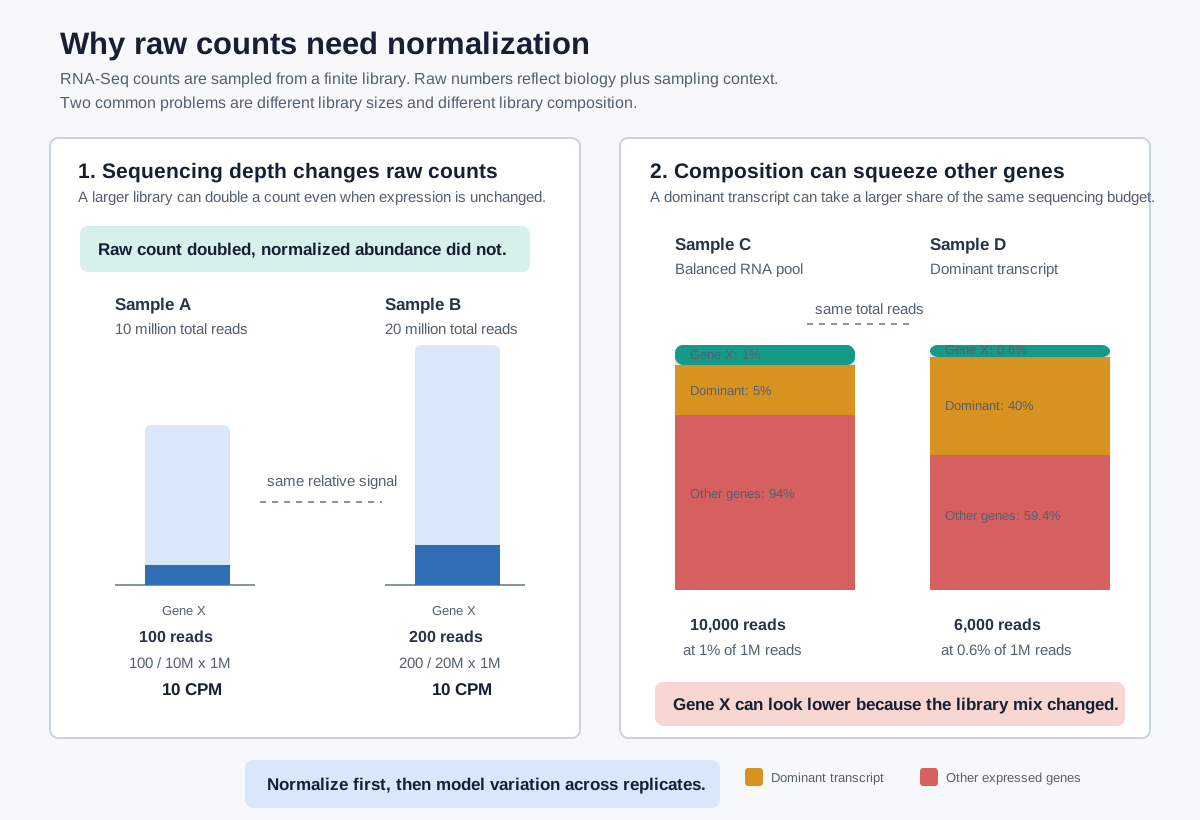
Figure: raw counts can change because sequencing depth changes, and they can also shift because one highly abundant transcript changes the composition of the finite sequencing library.
A Small Composition Example
Imagine two samples sequenced to exactly 1,000,000 reads. Gene X is upregulated in sample B. The library is fixed size, so other genes occupy a smaller fraction of the library even if their absolute molecule numbers did not change.
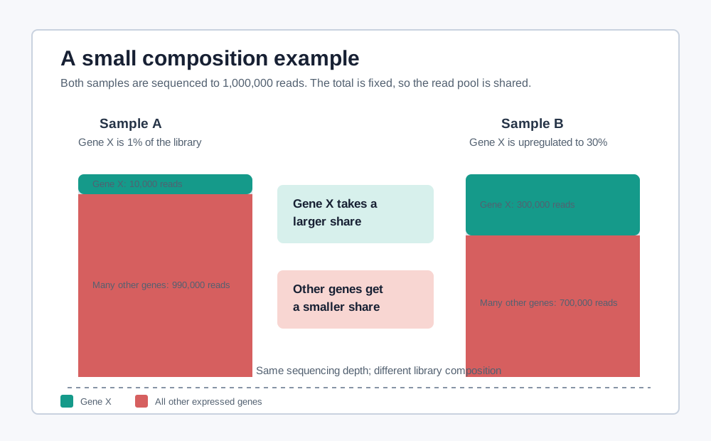
| Gene group | Sample A reads | Sample B reads | Naive interpretation |
|---|---|---|---|
| Gene X | 10,000 | 300,000 | Upregulated |
| Many unchanged genes | 990,000 | 700,000 | Appears downregulated |
This is why RNA-Seq normalization is not just "divide by total reads." Composition-aware methods try to estimate the sample scaling factor from genes that are not dominated by extreme expression changes.
4. QC Before DEG Analysis
Before DEG testing, we need to check that the count matrix and sample metadata are consistent, that library sizes are reasonable, and that biological replicates cluster together. If these checks fail, you should investigate and fix the problem before trusting downstream results.
If QC is skipped, DEG results are often misleading regardless of method.
Wrangling our count matrix
Different tools may expect our data to be in different formats. Does the method / tool require certain column names, a specific file type, or a particular orientation of the matrix? Check the documentation for your method of choice before starting. You may need to transpose the matrix, rename columns, or convert to a different file type using excel, R, or Python. You can also use genAI to help you write a script to reformat your count matrix.
Pre-DEG QC Checklist
-
Check sample metadata first
- Confirm sample labels match the count matrix.
- Verify condition names, replicate IDs, and batch variables.
- Make sure there are enough biological replicates (preferably at least 3 per group).
Replicate #
The number of replicates is of greater importance than the sequencing depth when applying differential expression methods. If you have a choice between sequencing more deeply or adding more replicates, adding replicates is usually the better choice. See Rapaport et al. 2013. Aim for 3-5 replicates per condition for a standard bulk RNA-seq experiment. More replicates are better, especially if you expect high biological variability.
-
Check sequencing depth and mapping summary
- Review total reads and mapped reads per sample.
- Flag samples with unusually low depth or low mapping rate.
- Ensure no sample is an extreme outlier in library size.
-
Check low-count burden
- Count how many genes have near-zero counts across all samples.
- Apply low-count filtering before DE testing.
- Record filtering criteria for reproducibility.
-
Check sample relationships
- Use PCA or MDS plots to inspect clustering.
- Use sample-to-sample correlation or distance heatmaps.
- Confirm biological replicates cluster more closely than unrelated samples.The experimental condition should be a major driver of separation in PCA or clustering.
Note
PCA, clustering, and correlation heatmaps are almost never run on raw counts. Raw counts have a mean-variance relationship that distorts distances between samples and can make clustering misleading, being largely driven by a few highly expressed genes. Instead, these plots should be built on log-transformed or variance-stabilized values (log2CPM, VST, or rlog). See Section 5 for how these are calculated.
-
Check for batch effects and outliers
- Ask whether batch, lane, date, or prep kit could drive separation in PCA.
- Investigate outlier samples before removing them.
- If batch effects are present, include batch terms in the design matrix.
-
Check normalization assumptions
- Ask whether most genes are expected to be unchanged.
- If massive global shifts are expected, note this as a limitation and consider spike-ins or external controls.
-
Check model readiness
- Confirm raw counts are used for DESeq2/edgeR/limma-voom workflows.
- Confirm contrast definitions are biologically meaningful.
- Confirm the final design matrix matches the experimental question.
Before we trust p-values, we trust QC. DEG is not a button click. If sample labels are wrong, replicates do not cluster, or batch dominates the data, your method choice will not save the analysis.
5. Normalization Strategies
Normalization adjusts for technical differences so that biological comparisons are more meaningful. It does not remove the need for replication, good experimental design, or statistical modeling.
Low-Count Filtering.
Filtering is not a normalization method, but like normalization, it is a preprocessing step that affects downstream results.
Before testing, low-count genes are usually filtered. Genes with almost no reads across the experiment provide little statistical power and increase the multiple-testing burden.
Filtering is not just cosmetic. It changes the set of genes being tested, which also affects downstream enrichment backgrounds.
CPM
Counts per million (CPM) divides each gene count by the total library size and multiplies by one million.
Use CPM for:
- quick expression summaries;
- low-count filtering;
- exploratory plots after appropriate transformations.
Do not treat simple CPM scaling as a complete DE model.
RPKM, FPKM, and TPM
RPKM/FPKM and TPM normalize for both gene length and sequencing depth.
- RPKM (Reads Per Kilobase per Million) and FPKM (Fragments Per Kilobase per Million) are length- and depth-normalized measures; FPKM is the paired-end version of RPKM.
- TPM (Transcripts Per Million) is similar but rescales values so all genes in a sample sum to one million, making within-sample comparisons more interpretable.
Use TPM-like values for:
- describing relative transcript abundance within a sample;
- comparing expression of different genes cautiously within one sample;
- some visualization and downstream signature-scoring contexts.
Do not use RPKM and FPKM, and avoid using RPKM/FPKM/TPM as direct input to DESeq2 or edgeR. Those packages are designed for count data and include their own between-sample normalization inside the model.
TMM
Trimmed Mean of M-values (TMM) is used by edgeR and is commonly used before limma-voom. It estimates scaling factors after trimming genes with extreme log fold changes or extreme abundance.
TMM is useful when library composition differs across samples because it avoids letting a small number of highly expressed genes define the scaling factor.
Median-of-Ratios / RLE
DESeq2 uses a median-of-ratios size factor approach. Each sample is compared to a pseudo-reference based on gene-wise geometric means, and the median ratio estimates the sample scaling factor.
This approach works well when most genes are not changing strongly in one direction. If nearly all genes truly shift in the same direction, any global-scaling method becomes difficult to interpret without spike-ins or an external reference.
Transformations for Plots
These are types of transformations not normalizations.
Normalization vs. transformation. - Normalization adjusts for differences in sequencing depth/library size between samples (e.g., converting to counts per million, CPM). - Transformation (log2, VST, rlog) stabilizes variance across the range of expression so that highly-expressed genes don't dominate downstream clustering.
Variance-stabilizing transformations (DESeq2::vst()), regularized log transforms (DESeq2::rlog()), and log2(CPM + c) (edgeR::cpm(log=TRUE)) are often used for:
- PCA;
- clustering;
- heatmaps;
- correlation plots.
These are usually visualization and exploratory-analysis transformations. They are not substitutes for the DE model used for p-values.
Note
rlog > vst > log2CPM in terms of variance stabilization, but rlog is slower to compute and can be memory-intensive for large datasets. VST is faster and more scalable, while log2CPM is the simplest and fastest, but less effective at stabilizing variance for low-count genes. All 3 are valid, and you can compare how well they stabilize variance in your own data by examining correlation scatterplots and mean-variance plots.
Want more information?
See https://hbctraining.github.io/Training-modules/planning_successful_rnaseq/lessons/sample_level_QC.html for a nice table comparing normalization strategies.
6. Meet the Tools
Before going further into theory, it helps to know what's actually out there. Three tools dominate RNA-Seq differential expression analysis in practice. All three are free, open-source, peer-reviewed, and distributed through Bioconductor, the main repository for genomics software in R. All three tools also have excellent documentation and active support communities, so consider reading the vignettes and tutorials for each tool for an in-depth understanding on how they work and how to use them. We only scratch the surface here.
Programming vs GUI
All three tools are R packages, but you do not need to know R to use them. iDEP (Integrated Differential Expression & Pathway analysis) provides a GUI that uses some of these tools under the hood. Running them directly in R gives you more flexibility, but requires some programming knowledge. You can start with iDEP and move to R later if you want more control. We will also see that iDEP provides R code snippets for each analysis, so you can learn the R commands while using the GUI and customize the code later if needed.
DESeq2
One of the two most widely used DE tools. Known for being relatively beginner-friendly with sensible defaults, strong documentation, and a very active support community.
- Bioconductor page: bioconductor.org/packages/DESeq2
- How it works: DESeq2 uses a "median-of-ratios" normalization strategy and models counts with a Negative Binomial distribution. It estimates per-gene dispersion and shrinks noisy estimates toward a global trend.
- Good first use case: A standard bulk RNA-seq comparison with a simple design and clear biological replicates.
edgeR
One of the two most widely used count-based DE tools, alongside DESeq2. Offers more manual control over the modeling process, but because of this, has a slightly steeper learning curve for beginners.
- Bioconductor page: bioconductor.org/packages/edgeR
- How it works: edgeR uses TMM normalization, fits Negative Binomial models with empirical Bayes dispersion estimation (often quasi-likelihood testing), and offers the most manual control for flexible, count-based modeling.
- Good first use case: Small-to-moderate studies where count-based modeling is preferred and the user wants flexibility.
limma-voom
Originally built for microarray data, extended to RNA-Seq counts via an added step called "voom." Particularly strong for complex experimental designs.
- Bioconductor page: bioconductor.org/packages/limma
- How it works: limma-voom typically uses TMM normalization then voom to convert counts to logCPM with precision weights, followed by weighted linear models with empirical Bayes moderation, making it especially strong for complex designs and multiple contrasts.
- Good first use case: Complex designs such as paired samples, batch-adjusted analyses, or multi-factor experiments.
Summary Table
Use this narrower 4-column version in Lesson8.md, replacing the current Summary Table.
| Method | Normalization + model (high level) | Best use case | Main tradeoff |
|---|---|---|---|
| DESeq2 | Median-of-ratios normalization; Negative Binomial GLM with shrinkage of dispersion (and optional log2FC shrinkage) | Standard two-group bulk RNA-seq with clear replicates | Strong defaults and robustness, but assumes most genes are not globally shifted |
| edgeR | TMM normalization; Negative Binomial modeling with empirical Bayes dispersion estimation (often quasi-likelihood testing) | Small-to-moderate studies needing flexible count-based modeling | Very flexible, but more manual choices can be harder for beginners |
| limma-voom | Usually TMM first, then voom converts counts to logCPM with precision weights; weighted linear models with empirical Bayes moderation | Complex designs (paired, batch-adjusted, multi-factor) and many contrasts | Powerful and fast, but depends on good mean-variance trend estimation and preprocessing |
Important Assumptions: All samples are correctly labeled and biologically independent; the input is raw count data; replication is available so biological variability can be estimated; and, via whichever normalization step each one relies on (median-of-ratios for DESeq2, TMM for edgeR and, typically, for limma-voom), that most genes are not changing dramatically in the same direction.
What Do the Comparison Studies Say?
No single method wins across every study, dataset, and sample size; multiple independent method-comparison papers agree on that much. EdgeR, DESeq2, and limma-voom all perform well in practice, as there are inconsistencies in benchmarking across studies, and most methods tend to converge on similar results at larger sample sizes. The choice of method is often less important than good experimental design, replication, and QC.
Here are a few sources to peruse if you want to dig deeper into the literature:
- Soneson & Delorenzi 2013 — simulation-based comparison of 11 DE methods
- Rapaport et al. 2013 — real-data benchmark using SEQC/ENCODE datasets.
- Seyednasrollah et al. 2015 — practical pipeline comparison of 8 packages
- Schurch et al. 2016 — 48-replicate yeast benchmark, with a focus on how many replicates you actually need
- Love 2016 blog post — a short, even-handed take from one of DESeq2's own authors on the DESeq2-vs-edgeR question
Why not just use a t-test?
RNA-Seq counts are discrete, non-negative integers with a large spike near zero and a long right tail, rather than the continuous, roughly bell-shaped data a t-test assumes. The simplest count model (Poisson, which assumes equal mean and variance) doesn't work either, because biological replicates vary more than Poisson allows, a property called overdispersion. DESeq2, edgeR, and limma-voom do not use exactly the same model, but they do solve the same RNA-Seq problems: extra variability beyond Poisson, small replicate numbers, and many near-zero genes. DESeq2 and edgeR use Negative Binomial count models, limma-voom uses weighted linear modeling of log-counts, and all three improve stability by sharing information across genes and by filtering sparse low-count features.
Why can't I find edgeR in iDEP?
DESeq2, edgeR, and limma-voom are the three tools you'll see referenced everywhere in the RNA-Seq literature, and all three are described above because you should know them. But when we move to iDEP in Lesson 2, you'll only find DESeq2, limma-voom, and limma-trend as DE testing options; edgeR is not one of them. iDEP does, however, quietly call edgeR's cpm() function under the hood for low-count filtering, so edgeR is present in the codebase, just not as a DE testing method you can select.
If your workflow specifically calls for edgeR, for example, matching a lab protocol, a collaborator's prior analysis, or a published method you're replicating, you'll need to run it separately in R or use a GUI that implements edgeR (e.g., Degust). iDEP remains an excellent way to get a fast, GUI-driven DESeq2 or limma-voom analysis, but it is not a drop-in replacement if edgeR specifically is required.
What About limma-trend?
You may see limma-trend listed as a fourth option in iDEP (and elsewhere). It's a close cousin of limma-voom, built on the same underlying limma package, but meant for a slightly different situation.
-
limma-voom takes raw counts, estimates the mean-variance trend, and turns it into a precision weight for every individual observation. It needs raw (or library-size-proportional) counts to do this correctly. Feeding it already-normalized values like TPM or CPM breaks its ability to infer the correct precision.
-
limma-trend takes the same kind of mean-variance trend but folds it into the statistical testing step itself (via the empirical Bayes moderation), rather than into per-observation weights. This makes it appropriate for already-normalized, log-scale expression data — including microarray data, or RNA-seq counts that have already been transformed to logCPM.
When to reach for limma-trend specifically: it's the simplest and most robust choice when sequencing depth (library size) is reasonably consistent across your samples. If library sizes vary a lot between samples, limma-voom is the more powerful choice, since it models that variability directly through its per-observation weights. When library sizes are similar, the two methods tend to give comparable results, and limma-trend is the lighter-weight option.
What If My Design Doesn't Fit Any of These?
DESeq2, edgeR, and limma-based methods cover most standard bulk RNA-Seq comparisons, but they're not the whole story. Specialized situations (e.g., single-cell RNA-Seq, longitudinal or repeated-measures designs, transcript-level (rather than gene-level) analysis, or experiments with very few or no replicates) often call for purpose-built methods beyond the scope of this lesson.
A good starting point for surveying what's out there is Conesa et al. 2016, "A survey of best practices for RNA-seq data analysis," Genome Biology. This review walks through experimental design, differential expression, and single-cell RNA-Seq considerations, and is a reasonable jumping-off point before searching for a method tailored to your specific design.
7. Going Further: R and Python
iDEP (Lesson 2) is a great way to run a first differential expression analysis without writing code. But a GUI can only take you so far, custom experimental designs, batch correction, multi-omics integration, and full reproducibility all eventually call for running DESeq2, edgeR, or limma-voom yourself, in R or Python.
If you're new to R, or want a refresher before tackling DE analysis in code, BTEP offers introductory training:
We also have singular lessons on specific topics like ClusterProfiler, ComplexHeatmap, ggpubr, Quarto, etc. in the BTEP Coding Club documentation. I recommend searching for "R Programming" in the BTEP Coding Club documentation to find relevant lessons.
Roughly, here's the path:
- Learn base R (or brush up) — vectors, data frames, reading in files.
- Learn to load a count matrix and sample metadata into R.
- Follow a DESeq2 or edgeR vignette on your own data (see the Bioconductor links in Section 3).
Python users can reach similar results with packages such as PyDESeq2, though the R ecosystem remains the most mature and best-documented path for RNA-Seq DE analysis today.
For an introduction to python, BTEP offers the Python Introductory Education Series.
8. Introducing iDEP
In the next lesson, we'll put everything from this lesson into practice using iDEP (integrated Differential Expression and Pathway analysis), a free, web-based tool that runs DESeq2, limma-voom, and limma-trend behind a point-and-click interface, so you can go from a count matrix to differential expression results and pathway enrichment without writing any code.
iDEP was built by the Ge Lab at South Dakota State University and is available as a public web app at bioinformatics.sdstate.edu/idep. For this training, we'll instead be running iDEP directly on Biowulf, NIH's HPC cluster, using version iDEP 2.01.
Running iDEP on Biowulf rather than the public web app has a few advantages for our purposes:
- Your data stays on NIH systems rather than being uploaded to an external server.
- You get dedicated compute resources rather than sharing a public server with other users worldwide.
Files and iDEP on Biowulf
The file browser in iDEP on Biowulf accesses your local file system (on your laptop or workstation) rather than the Biowulf file system. You can either download the count matrix to your local machine and upload it to iDEP, or mount the Biowulf file system on your local machine and upload the count matrix from there.
What You'll Need
- An active Biowulf account (see https://hpc.nih.gov/docs/accounts.html if you don't have one yet). Student accounts are available to a limited number of registrants for this training.
- Access to the NIH network or VPN.
- Your count matrix file (from Section 1 —
RSEM.genes.expected_count.all_samples.txtor your own data, formatted the same way).
Getting the Data
You can download the count matrix here.
9. Accessing iDEP via HPC Open OnDemand on Biowulf
Step 1 — Log in to HPC Open OnDemand
- Navigate to https://hpcondemand.nih.gov/ (NIH network or VPN required).
- Authenticate with your NIH credentials (PIV/MFA).
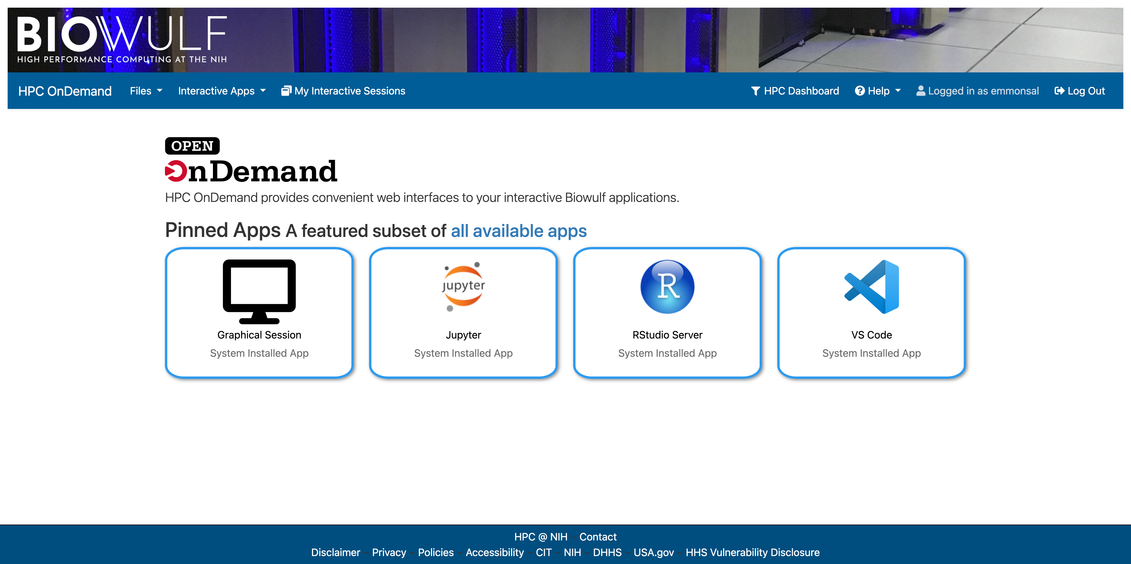
HPC Open OnDemand Dashboard at login.
Student Accounts
A limited number of student accounts are available for this lesson. If you are using a student account, navigate to https://hpcclass.cit.nih.gov/. If you were not able to grab a student account and you do not have a Biowulf account, feel free to use the public iDEP server.
Step 2 — Launch the iDEP app
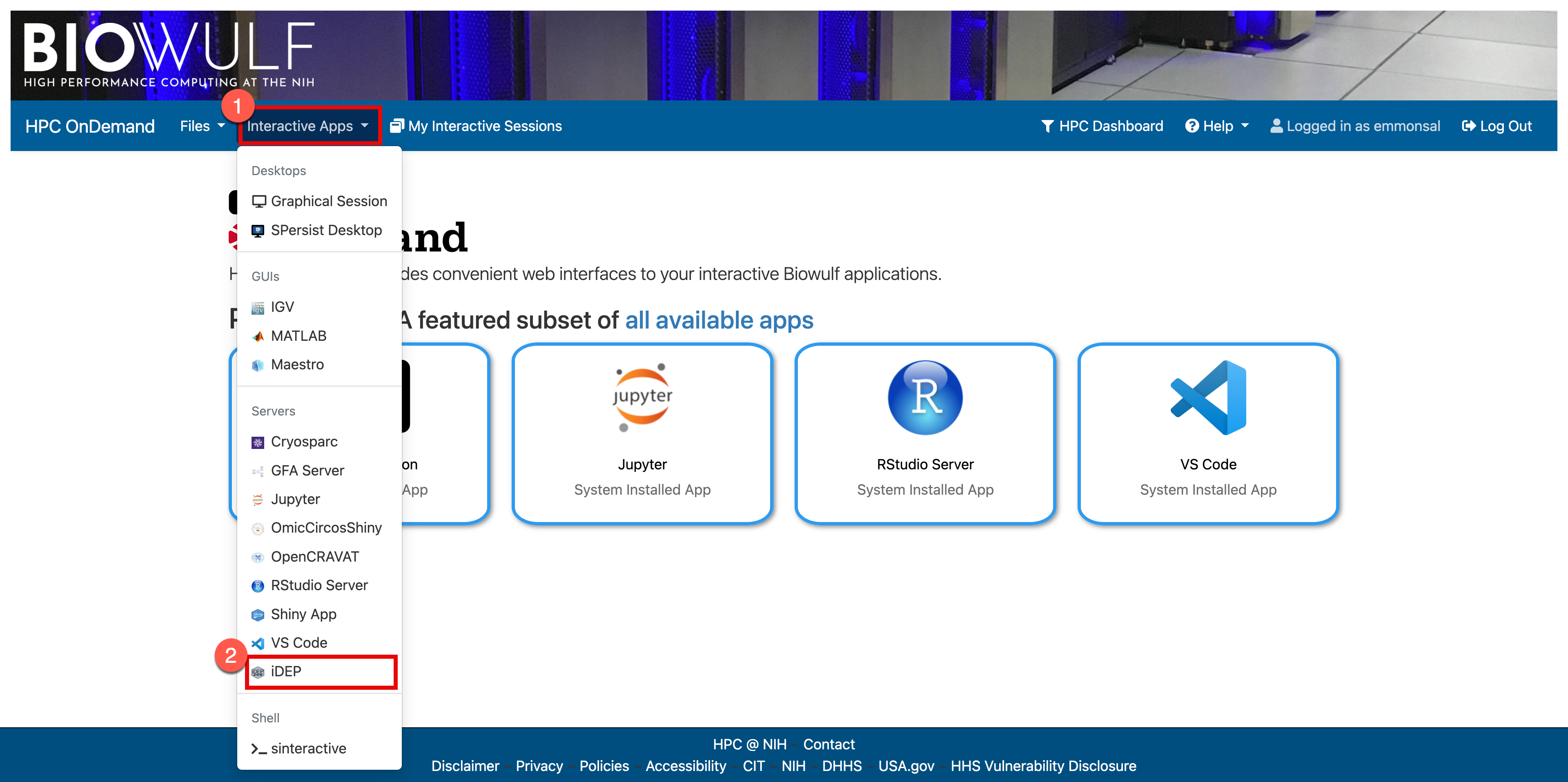
iDEP is not among the four pinned apps on the OnDemand homepage, but it is available in the full list of interactive applications.
- From the Open OnDemand dashboard, locate the "Interactive Apps" tab and select iDEP.
- Select appropriate resource parameters for your session (CPUs, memory, walltime)
- Launch the session and wait for the job to be allocated on a compute node.
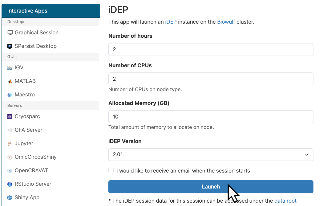
Select resources for your iDEP session and launch the job.
Step 3 — Connect to your running iDEP session
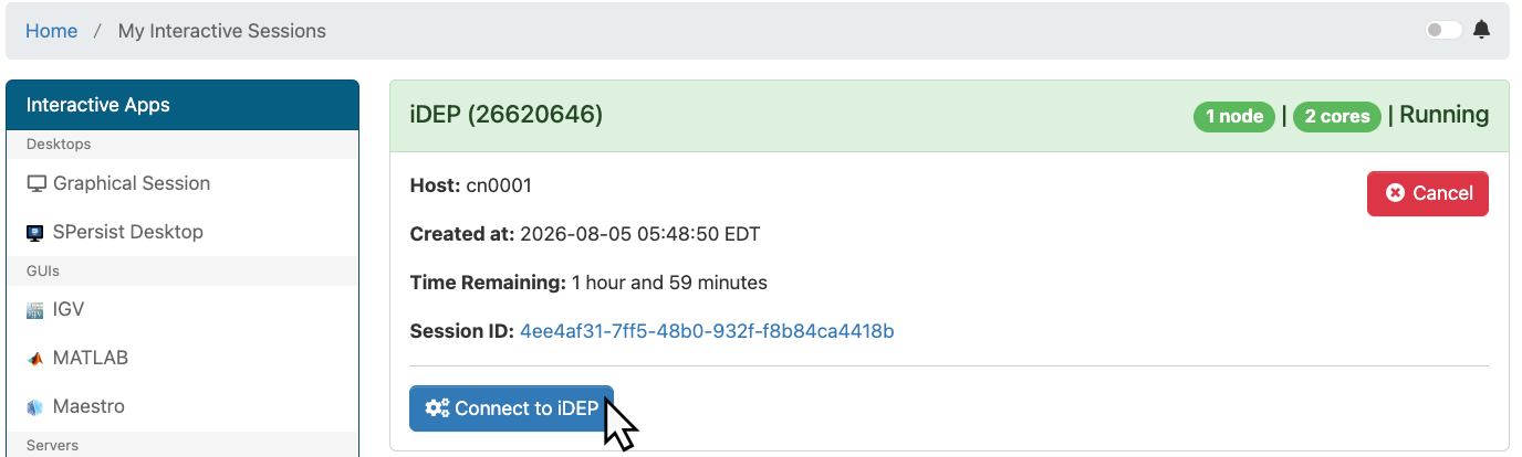
- Once the job starts, Open OnDemand will provide a Connect to iDEP button/link.
- This opens the iDEP Shiny interface directly in your browser — no manual SSH tunneling required.
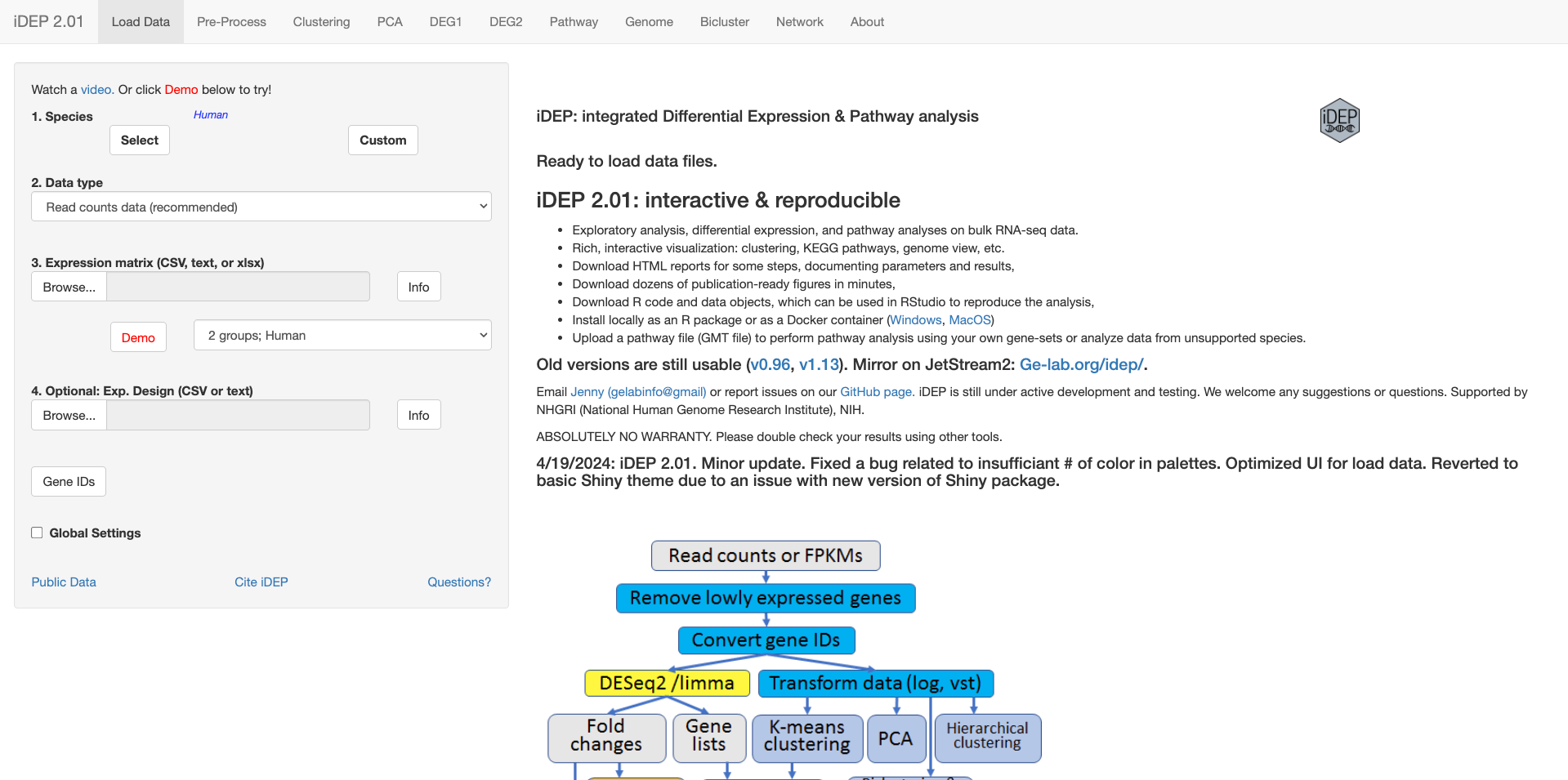
Step 4 — Orient yourself in the iDEP interface
Step 5 — Upload your count matrix
There is no way to save the current iDEP session, so you will need to upload your count matrix (or other accepted files) each time you start a new session. We will walk through the upload process in Lesson 2, but here are some important points to keep in mind:
- The gene expression matrix must be a tab-delimited or comma separated value file with rows as genes and columns as samples. The first column should contain gene identifiers, and the first row should contain sample identifiers. See the Data Format section of the iDEP documentation for details: https://idepsite.wordpress.com/data-format/.
- iDEP can convert gene identifiers to Ensembl IDs for many species, but it is best to use Ensembl IDs in your input file if possible.
- Ensemble IDs should not include version numbers (e.g., ENSG00000123456.1). If your input file has version numbers, you can remove them in R or Python before uploading.
- The raw count matrix must contain integer counts. RSEM outputs non-integer expected counts, so you will need to round them to integers before uploading. iDEP will not accept non-integer counts.
How can I wrangle my input file without programming experience?
- You can use Excel or Google Sheets to remove version numbers, transpose the matrix, or rename columns.
- You can also use genAI to reformat your count matrix.
Example prompt:
I have a tab-delimited count matrix that needs to be reformatted for iDEP differential expression analysis.
Please apply the following changes and save the result as [output_filename].txt:

1. Remove the GeneName column entirely.
2. Keep the gene_id column and its header, but strip any version suffixes from the IDs
(e.g. ENSG00000276871.1 → ENSG00000276871).
3. Round all numeric data columns to integers.

The file will always contain gene_id and GeneName columns. The number and names of the numeric
data columns may vary. Please make no other changes to the file.

The input file is attached: [input_filename].txt.
Alternatively, you can use AI to generate a script in R or Python that performs the same operations on your count matrix, and use that script as a reusable tool for future datasets and a record for reproducibility.
Please draft an R script that can implement the changes that were applied to test.txt. The script should be able to take any similarly formatted file. You can expect the gene_id and GeneName columns to be in any file acted on by the script, but the columns with numeric data will not have variable names. There may also be 1 or more numeric data columns. Please make the script robust but simple.
Version differences between iDEP on Biowulf and the public web app
iDEP on Biowulf is currently version 2.01, which may differ slightly in menu layout from the public web app at bioinformatics.sdstate.edu/idep, which is on a newer release. If something doesn't match a tutorial you find online, check the version number first.
In lesson 2, we will start with a wrangled count matrix and walk through the iDEP interface to run a full differential expression analysis. You can find our wrangled count matrix here.
10. Quick Knowledge Check
1. Why is a raw count of 200 in one sample not automatically higher expression than a raw count of 100 in another sample?
Library size, composition, and other technical factors can differ across samples.
2. Why are TPM values useful for description but not ideal as direct input to DESeq2 or edgeR?
TPM values are useful for viewing relative abundance, but count-based DE methods expect raw counts and do their own normalization.
3. Why should QC be done before DEG testing?
QC catches problems (mislabels, outliers, batch effects, poor depth) that can invalidate downstream results.
4. What does a positive log2 fold change mean?
The gene is estimated to be higher in the comparison group than in the reference group.
5. Why do we adjust p-values when testing thousands of genes?
Testing many genes creates false positives by chance, so p-values must be adjusted.
6. Name one sign from PCA or sample correlation that tells you DEG results may not be trustworthy yet.
Example answers: replicates do not cluster together, one sample is an extreme outlier, or samples separate by batch instead of biology.
7. Name the three major DE tools and one distinguishing "good first use case" for each.
DESeq2 (standard two-group comparisons), edgeR (flexible count modeling for small-to-moderate studies), limma-voom (complex/multi-factor designs).
Which of the three major DE tools is not available as a DE testing method in iDEP, and why?
edgeR. iDEP's developers built DE testing around limma-trend, limma-voom, and DESeq2, and explicitly left edgeR as a possible future addition.
Take-Home Messages
- DE analysis tests whether expression differences are larger than chance — it is not a ranking of raw counts. Interpret effect size and adjusted p-value together.
- DESeq2, edgeR, and limma-voom are the three tools you'll meet everywhere — all free, peer-reviewed, and available through Bioconductor.
- Always use raw counts as input to DESeq2, edgeR, and limma-voom. TPM and FPKM values are not appropriate inputs for these tools.
- Normalization assumes most genes are not changing. QC before testing is the best way to check that this assumption holds.
- No statistical method can rescue poor experimental design or missing replicates.
- iDEP (next lesson) gets you a full analysis with no code — using DESeq2 and limma-based methods. If your workflow specifically requires edgeR, you'll need to run it separately in R.
- R or Python gives you full flexibility once you're ready for it, including access to every method mentioned in this lesson.
Recommended Reviews and Tutorials by Section
Resources Used
- Love MI, Huber W, Anders S. 2014. Moderated estimation of fold change and dispersion for RNA-seq data with DESeq2. Genome Biology. https://doi.org/10.1186/s13059-014-0550-8
- DESeq2 Bioconductor package and vignette: https://bioconductor.org/packages/DESeq2/
- Robinson MD, McCarthy DJ, Smyth GK. 2010. edgeR: a Bioconductor package for differential expression analysis of digital gene expression data. Bioinformatics. https://doi.org/10.1093/bioinformatics/btp616
- edgeR Bioconductor package and user guide: https://bioconductor.org/packages/edgeR/
- Law CW, Chen Y, Shi W, Smyth GK. 2014. voom: precision weights unlock linear model analysis tools for RNA-seq read counts. Genome Biology. https://doi.org/10.1186/gb-2014-15-2-r29
- Smyth GK. 2004. Linear models and empirical Bayes methods for assessing differential expression in microarray experiments. Statistical Applications in Genetics and Molecular Biology. https://doi.org/10.2202/1544-6115.1027
- limma Bioconductor package: https://bioconductor.org/packages/limma/
- Brintha VPB. LinkedIn post: "DESeq2, edgeR, and limma-voom are among the most widely used methods..." — Accessible visual summary of the three-stage comparison framework (variance modeling, expression modeling, statistical testing). https://www.linkedin.com/posts/brintha-vpb_deseq2-edger-and-limma-voom-are-among-the-share-7469552632911683584-OnDu/
- Robinson MD, Oshlack A. 2010. A scaling normalization method for differential expression analysis of RNA-seq data. Genome Biology. https://doi.org/10.1186/gb-2010-11-3-r25
- Zhao S et al. 2020. Misuse of RPKM or TPM normalization when comparing across samples and sequencing protocols. RNA. https://doi.org/10.1261/rna.074922.120
- iDEP web application documentation, verified June 8, 2026: https://bioinformatics.sdstate.edu/idep/
- Ge SX, Son EW, Yao R. 2018. iDEP: an integrated web application for differential expression and pathway analysis of RNA-Seq data. BMC Bioinformatics 19:534. https://doi.org/10.1186/s12859-018-2486-6 (states that DE testing in iDEP uses limma-trend, limma-voom, and DESeq2, noting edgeR may be incorporated in the future)
- iDEP on Biowulf (NIH HPC), version 2.01, verified July 2026: https://hpc.nih.gov/apps/idep.html
- NIH HPC Open OnDemand documentation, verified July 2026: https://hpc.nih.gov/ondemand/
- Conesa A et al. 2016. A survey of best practices for RNA-seq data analysis. Genome Biology. https://doi.org/10.1186/s13059-016-0881-8
- Soneson C, Delorenzi M. 2013. A comparison of methods for differential expression analysis of RNA-seq data. BMC Bioinformatics. https://pmc.ncbi.nlm.nih.gov/articles/PMC3608160/
- Evans C, Hardin J, Stoebel DM. 2018. Selecting between-sample RNA-Seq normalization methods from the perspective of their assumptions. Briefings in Bioinformatics. https://pmc.ncbi.nlm.nih.gov/articles/PMC6171491/
- Dillies MA et al. 2013. A comprehensive evaluation of normalization methods for Illumina high-throughput RNA sequencing data analysis. Briefings in Bioinformatics. https://doi.org/10.1093/bib/bbs046
- Rapaport F et al. 2013. Comprehensive evaluation of differential gene expression analysis methods for RNA-seq data. Genome Biology. https://doi.org/10.1186/gb-2013-14-9-r95
- RNA-seq workflow: gene-level exploratory analysis and differential expression. Bioconductor. https://bioconductor.org/packages/release/workflows/vignettes/rnaseqGene/inst/doc/rnaseqGene.html
- RNA-seq analysis is easy as 1-2-3 with limma, Glimma and edgeR. Bioconductor. https://www.bioconductor.org/packages/devel/workflows/vignettes/RNAseq123/inst/doc/limmaWorkflow.html
- edgeR quasi-likelihood RNA-seq workflow. Bioconductor. https://bioconductor.posit.co/packages/3.19/workflows/vignettes/RnaSeqGeneEdgeRQL/inst/doc/edgeRQL.html
- Harvard FAS Informatics Group. Bulk RNA-seq DE analysis tutorial. https://informatics.fas.harvard.edu/resources/tutorials/differential-expression-analysis/
- Anders S, Huber W. 2010. Differential expression analysis for sequence count data. Genome Biology. https://doi.org/10.1186/gb-2010-11-9-r106
- McCarthy DJ, Chen Y, Smyth GK. 2012. Differential expression analysis of multifactor RNA-Seq experiments with respect to biological variation. Nucleic Acids Research. https://doi.org/10.1093/nar/gks042
- Bourgon R, Gentleman R, Huber W. 2010. Independent filtering increases detection power for high-throughput experiments. PNAS. https://doi.org/10.1073/pnas.0914005107
- HBC Training. Introduction to DGE (archived). https://hbctraining.github.io/DGE_workshop/lessons/01_DGE_setup_and_overview.html