Differential Alternative Splicing Analysis with rMATS
Learning Objectives
After this class, the participants will be able to:
- Understand the capabilities of RMATS in the context of differential alternative splicing events detection
- Use Biowulf "rMATS" module to analyze their RNAseq data
- OPTIONAL: Visualize the output using "rmats2sashimiplot" software package
What is Alternative Splicing?
Alternative splicing is a crucial molecular process within eukaryotic cells whereby precursor messenger RNA (pre-mRNA) molecules are selectively modified, resulting in the production of multiple distinct mRNA transcripts from a single gene. This process allows cells to diversify their gene expression and generate various protein isoforms with different functions or properties, thereby contributing to the complexity and versatility of biological systems.
Alternative splicing was first discovered in the early 1970s. The landmark discovery was made by the scientists Richard J. Roberts and Phillip A. Sharp, who were awarded the Nobel Prize in Physiology or Medicine in 1993 for their groundbreaking work.
Types of Alternative Splicing
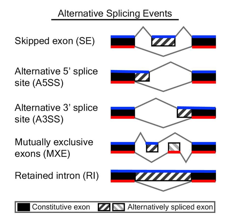
Modified from: https://rnaseq-mats.sourceforge.io
Note
Sometimes "Alternative Promoters" and "Alternative polyadenylation" are classified as additional types of alternative splicing
Methods and Packages
RSEM
https://bmcbioinformatics.biomedcentral.com/articles/10.1186/1471-2105-12-323
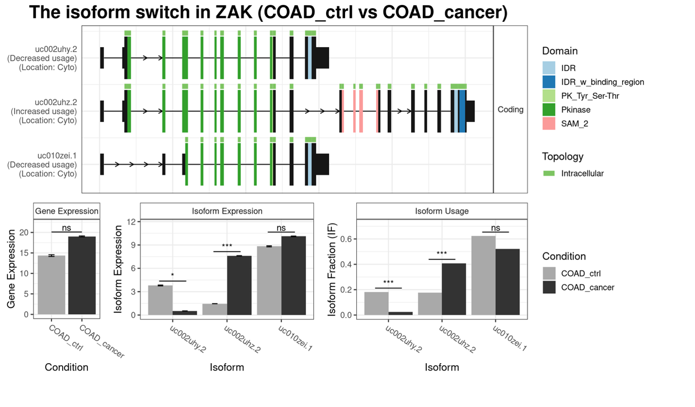
IsoformSwitchAnalyzeR
https://bioconductor.org/packages/release/bioc/html/IsoformSwitchAnalyzeR.html
DEXSeq
https://bioconductor.org/packages/release/bioc/html/DEXSeq.html
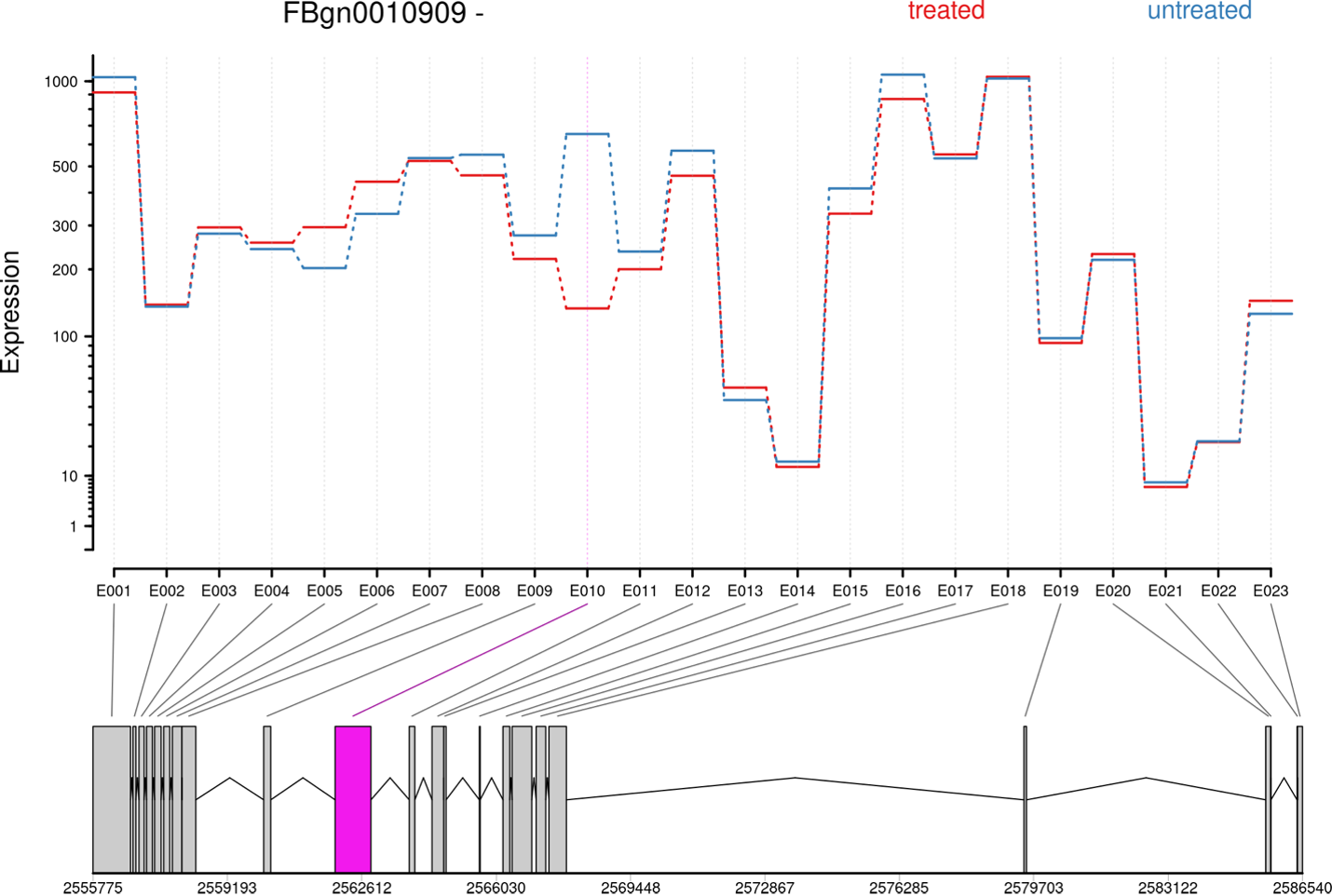
These tools serve different purposes within the RNA-Seq analysis workflow. rMATS (that would be discussed today) is tailored for identifying differential alternative splicing events, IsoformSwitchAnalyzeR focuses on isoform-level differential expression, and DEXseq specifically detects differential exon usage. The choice between them depends on the specific research questions and goals of your RNA-Seq analysis.
What is rMATS?
rMATS is a computational tool for detection and quantification of differential alternative splicing events. rMATS stands for "replicate Multivariate Analysis of Transcript Splicing". After its initial release in 2011, it saw continuous development and improvement, with the most recent version (as of September 2023) being rMATS turbo 4.1.2
- Purpose: rMATS is primarily used for the detection and quantification of differential alternative splicing events between two or more conditions.
- Key Features: It focuses on splicing events like exon skipping, alternative 5' and 3' splice site usage, and intron retention.
- Output: Provides information about the type and significance of splicing changes.
- Applications: rMATS is particularly useful for studying how alternative splicing varies between conditions or treatments.
rMATS analysis has two steps, prep and post. The idea was to make it possible to run computationally intensive first step on different machines simultaneously, and then merge the results during the final step. Also, the rMATS statistical model can be run independently, which can be useful when there are more than two groups to compare. By default, both steps (prep + post, which includes stat) would be run.
Installation notes
Please note that rMATS was tested only with Linux (though it can be compiled for MacOS, if some modifications are made).
rMATS can be installed and run locally, if the following dependencies are satisfied:
- Python (3.6.12 or 2.7.15)
- Cython (0.29.21 or 0.29.15 for Python 2)
- numpy (1.16.6 or 1.16.5 for Python 2)
- BLAS, LAPACK
- GNU Scientific Library (GSL 2.5)
- GCC (>=5.4.0)
- gfortran (Fortran 77)
- CMake (3.15.4)
- PAIRADISE (optional)
- Samtools (optional)
- STAR (optional)
There is an option to create conda environment for Python and R
dependencies, if --conda flag is used with build_rmats script.
Alternatively, a docker version is also available, which can be run by using the following command:
docker run rmats:turbo01 [options]
However, taking into consideration resources required to run the analysis, it is recommended to utilize the version preinstalled on Biowulf:
A link to rMATS documentation on Biowulf:
https://hpc.nih.gov/apps/rMATS.html
Running rMATS on Biowulf
The program can be run in either interactive or batch mode
Get interactive node:
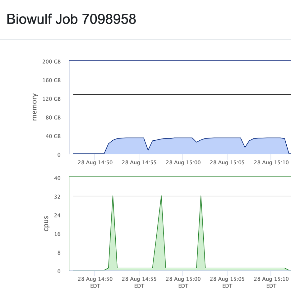
sinteractive -c 16 --mem 45g --gres=lscratch:20
Make sure you have requested enough resources, as the program can be quite memory- and CPU-hungry
Note
A comment: behind the scene, a STAR aligher (by Alexander Dobin) is used. So, essentially, the requirements are set by STAR. Thus, to align reads to a mammalian genome (human or mouse), 30-40GB of available RAM would be required.
Prepare your data
You will need an annotation file in GTF format (for poorly annotated species you can use GTF file generated by cufflinks). ENSEMBL annotation is known to work well.
Additionally, a STAR index (for appropriate STAR version) is required if FASTQ files are used as input.
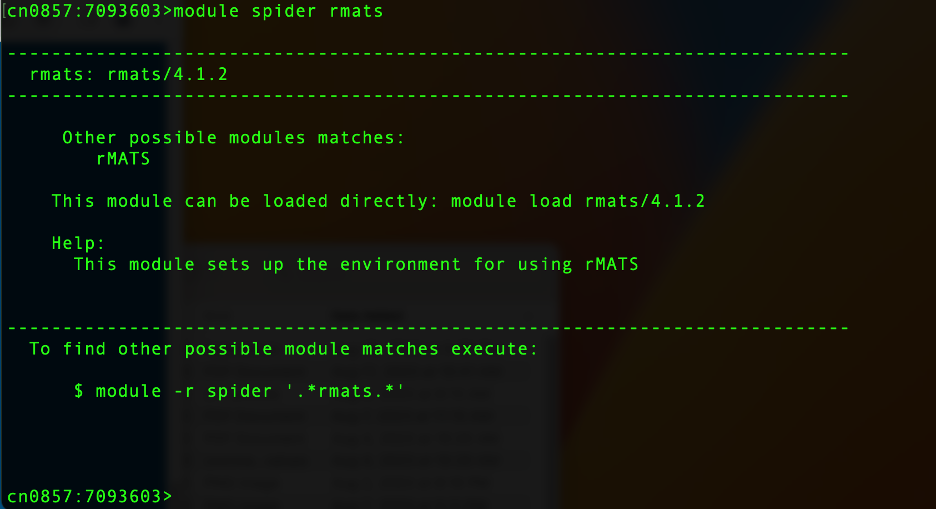
Load required module. Please note that newer versions might be available in the future, so while a command listed on Biowulf page would work:
module load rmats/4.1.2
It might be more efficient to use shorter version:
ml rmats
(ml here works as a shortcut for module load; using "rmats" without
specifying a version loads the default [usually the latest] version)
Prepare your input files. If you are using raw FASTQ files, then list all samples of one group in one TXT file:
231ESRP.25K.rep-1.R1.fastq:231ESRP.25K.rep-1.R2.fastq,231ESRP.25K.rep-2.R1.fastq:231ESRP.25K.rep-2.R2.fastq
And all samples of another group in another file:
231EV.25K.rep-1.R1.fastq:231EV.25K.rep-1.R2.fastq,231EV.25K.rep-2.R1.fastq:231EV.25K.rep-2.R2.fastq
Note
Please note that samples within the same group are separated by comma (","), and if you have a paired-end sequences they are separated by colon (":") in R1:R2 format.
Now you are ready to run your analysis:
rmats.py --s1 $PWD/s1.txt --s2 $PWD/s2.txt --gtf \
gtf/Homo_sapiens.Ensembl.GRCh37.72.gtf --bi \
/fdb/STAR_indices/2.7.8a/GENCODE/Gencode_human/release_27/genes-100 \
--od out_test -t paired --nthread $SLURM_CPUS_PER_TASK --readLength \
50 --tophatAnchor 8 --cstat 0.0001 --tstat 6 --tmp \
/lscratch/${SLURM_JOB_ID}
Let's analyze the command pasted above.
In our example, we are using rMATS version 4.1.2 (currently, the only
version available on Biowulf), and rmats.py is the main executable
file. Keep in mind, that it might change in the future versions -- some
of earlier releases required the user to run python rmats.py or just
`rmats``.
Here, we have 2 groups of samples, with information about the first
group is stored in a file named "s1.txt", located in the current working
directory ($PWD), and the information about the second group is stored
in a file "s2.txt". The content of these text files is listed above, in
a section titled "Prepare your input files". A flag --s1/--s2 is
used to indicate that raw data (=FASTQ files) are being used as input;
for BAM files, these flags would be --b1/--b2. File names for
FASTQ or BAM files could also be used directly in a command line, but
that decrease the readability and may result in a typo, so preparing
s1.txt/s2.txt (or their analogs for BAM files) is generally recommended.
Note
A comment: Historically, rMATS required all reads to have the same length, and most BAM files coming from other sources contained variable-length reads (some trimmed during pre-processing step, to remove adapter or lower-quality bases; some soft- or hard-clipped during alignment stage). The rationale for this requirement was that statistical model was based on the assumption of equal lengths of all reads, so any variation in length made calculated p-values invalid. So, in most cases, using original (untrimmed) FASTQ files to generate a new alignment was the best choice.
The following two parameters, --gtf and --bi, provide information
about genome annotation (in GTF format) and STAR index (needed for
alignment). Please keep in mind that index you provide needs to be
compatible with STAR version used by the program.
The --od parameter lets you specify the name (and location) of the
output folder, where information about identified splicing events would
be kept.
-t (note a single dash here) and --readLength parameters are
describing your sequencing data: paired or single, and the length of
each read. It is also recommended to specify the library type, if known,
using --libType parameter (by default, the program treats data as
unstranded)
--nthread, --tstat and --tmp parameters are used to specify
computational resources available for this job: the number of
processors/threads, the number of threads for statistical model and the
location for temporary files. These can be specified explicitly (as
Biowulf team did for tstat); but using system variables such as
"$SLURM_CPUS_PER_TASK" is an elegant way to "set it once and never
worry about this again".
The cutoff value for splicing difference is specified by --cstat
parameter. The default value of 0.0001 corresponds to 0.01% difference.
--tophatAnchor parameter applies only if FASTQ files are used, and
specifies the "anchor length" (also called "overhang length") -- a
number of nucleotides that must be mapped to each end of a given
junction.
Full list of available parameters can be found using the following command:
rmats.py -h
or
rmats.py --help
Note
There are some variations between different versions of rMATS.
rMATS output format
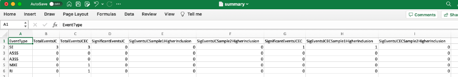
Output folder (specified by --od parameter) will contain files for
each type of splicing event (marked as RI for "retained intron", SE for
"skipped exon", A3SE for "alternative 3' splice site", A5SE for
"alternative 5' splice site", MXE for "mutually exclusive exons") in TXT
format.
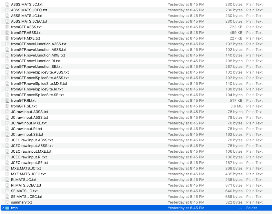
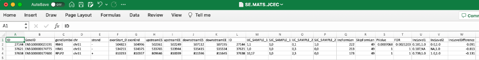
Files with extension .MATS.JC.txt include only reads that span junctions (Junction Counts); with extension .MATS.JCEC.txt include both reads that span junctions and reads that do not cross an exon boundary (Exon Counts). These are the final output files, containing coordinate information, counts, FDR and p-value -- thus, making them most useful for us:
Files starting with "fromGTF." contain all identified splicing evens derived from GTF and RNA (coordinates only):

Files with ".raw.input." in the file name include event counts for junctions only (JC) or junctions and exons (JCEC) -- counts only:
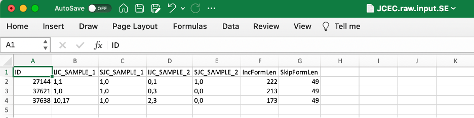
The following description of output format is provided in rMATS manual:
-
Shared columns:
-
ID: rMATS event id
-
GeneID: Gene id
-
geneSymbol: Gene name
-
chr: Chromosome
-
strand: Strand of the gene
-
IJC_SAMPLE_1: Inclusion counts for sample 1. Replicates are comma separated
-
SJC_SAMPLE_1: Skipping counts for sample 1. Replicates are comma separated
-
IJC_SAMPLE_2: Inclusion counts for sample 2. Replicates are comma separated
-
SJC_SAMPLE_2: Skipping counts for sample 2. Replicates are comma separated
-
IncFormLen: Length of inclusion form, used for normalization
-
SkipFormLen: Length of skipping form, used for normalization
-
PValue: Significance of splicing difference between the two sample groups. (Only available if the statistical model is on)
-
FDR: False Discovery Rate calculated from p-value. (Only available if statistical model is on)
-
IncLevel1: Inclusion level for sample 1. Replicates are comma separated. Calculated from normalized counts
-
IncLevel2: Inclusion level for sample 2. Replicates are comma separated. Calculated from normalized counts
-
IncLevelDifference: average(IncLevel1) - average(IncLevel2)
-
-
Event specific columns (event coordinates):
-
SE: exonStart_0base exonEnd upstreamES upstreamEE downstreamES downstreamEE
- The inclusion form includes the target exon (exonStart_0base, exonEnd)
-
MXE: 1stExonStart_0base 1stExonEnd 2ndExonStart_0base 2ndExonEnd upstreamES upstreamEE downstreamESdownstreamEE
-
If the strand is + then the inclusion form includes the 1st exon (1stExonStart_0base, 1stExonEnd) and skips the 2nd exon
-
If the strand is - then the inclusion form includes the 2nd exon (2ndExonStart_0base, 2ndExonEnd) and skips the 1st exon
-
-
A3SS, A5SS: longExonStart_0base longExonEnd shortES shortEE flankingES flankingEE
- The inclusion form includes the long exon (longExonStart_0base, longExonEnd) instead of the short exon (shortESshortEE)
-
RI: riExonStart_0base riExonEnd upstreamES upstreamEE downstreamES downstreamEE
- The inclusion form includes (retains) the intron (upstreamEE, downstreamES)
-
Finally, a summary file provides the overview of the results:
OPTIONAL: Visualizing rMATS output
Getting rmats2sashimiplot
git clone https://github.com/Xinglab/rmats2sashimiplot/
No installation required; however, conversion from Python2 to Python3 might be needed:
./rmats2sashimiplot/2to3.sh
To run the program, use "python" command with a path:
python ./src/rmats2sashimiplot/rmats2sashimiplot.py
Here is an example of a command to be used with results of Biowulf's test run:
python rmats2sashimiplot/src/rmats2sashimiplot/rmats2sashimiplot.py \
-o PIC --b1 b1.txt --b2 b2.txt --event-type SE \
-e default-out/SE.MATS.JC.txt --l1 SampleOne --l2 SampleTwo \
--color '#CC0011,#CC0011,#FF8800,#FF8800'
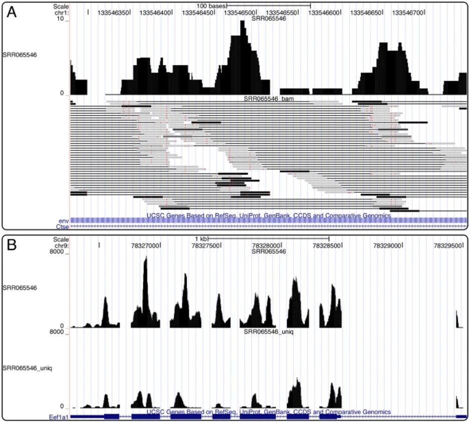
Visualizing Biowulf example results:
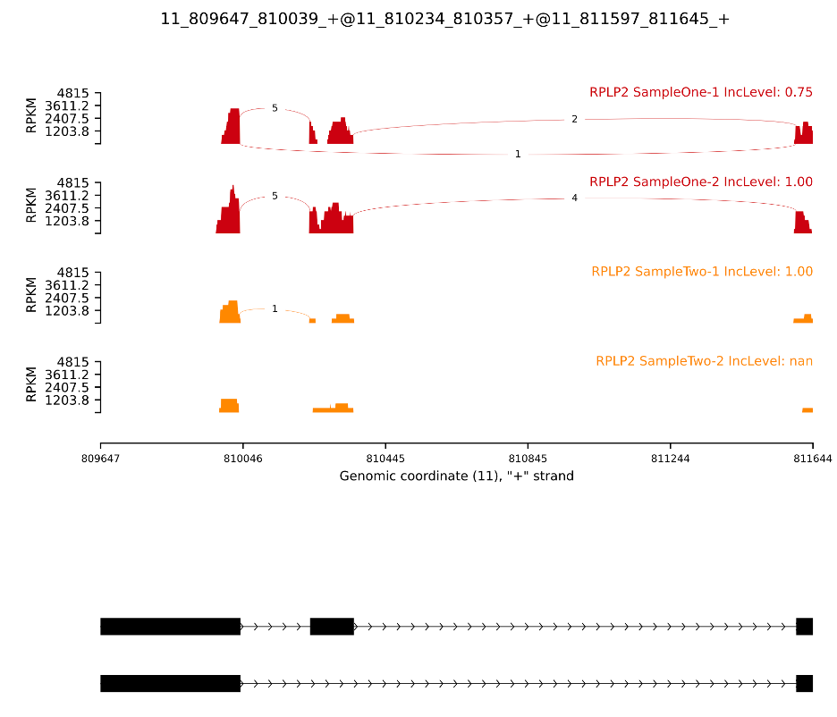
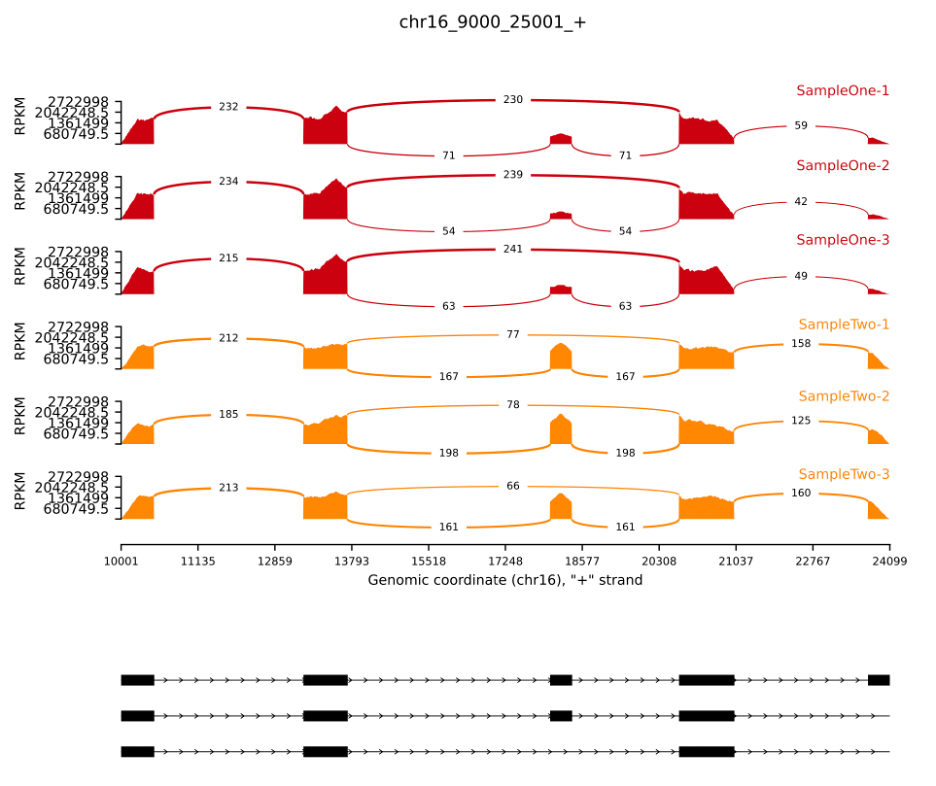
Unfortunately, this dataset was optimized for testing purposes, so it doesn't allow us to generate a nice-looking image. Let's try an example provided by the authors instead:
Command used:
python rmats2sashimiplot/src/rmats2sashimiplot/rmats2sashimiplot.py  --b1 \
./rmats2sashimiplot_test_data/sample_1_replicate_1.bam,\
./rmats2sashimiplot_test_data/sample_1_replicate_2.bam,\
./rmats2sashimiplot_test_data/sample_1_replicate_3.bam --b2 \
./rmats2sashimiplot_test_data/sample_2_replicate_1.bam,\
./rmats2sashimiplot_test_data/sample_2_replicate_2.bam,\
./rmats2sashimiplot_test_data/sample_2_replicate_3.bam \
-c chr16:+:9000:25000:./rmats2sashimiplot_test_data/annotation.gff3 \
--l1 SampleOne --l2 SampleTwo --exon_s 1 --intron_s 5 \
-o test_coordinate_output
And here is the result:
References:
rMATS publications
https://www.pnas.org/doi/full/10.1073/pnas.1419161111
https://link.springer.com/protocol/10.1007/978-1-62703-514-9_10
https://academic.oup.com/nar/article/40/8/e61/2411737
rMATS web page
https://rnaseq-mats.sourceforge.io
rMATS on Biowulf
https://hpc.nih.gov/apps/rMATS.html
rmats2sashimiplot web page
https://github.com/Xinglab/rmats2sashimiplot