VLOOKUP in excel and the R programming equivalent
Introducing the BTEP Coding Club
The BTEP Coding club is a new initiative to provide more tailored bioinformatics training to the NCI community. Each month we will feature a 1-hour demo / tutorial of a bioinformatics tool, software, skill, or platform.
We welcome suggestions from the NCI community. Email us at ncibtep@nih.gov if there is a specific topic you would like to see featured.
Learning Objectives.
- Learn how to use the VLOOKUP function.
- Discuss advantages and disadvantages of using Excel.
- Demonstrate similar VLOOKUP functionality with R programming.
- Discuss advantages / disadvantages of using R and resources to continue R learning.
What is VLOOKUP?
VLOOKUP is an excel function that performs vertical look-ups, or look up by row across columns.
The two main purposes of VLOOKUP are to:
- find a result in your data by using a key in another column and
- to merge tables.
Info
In 2019, Excel introduced the function XLOOKUP to succeed VLOOKUP and HLOOKUP. XLOOKUP works similarly but gets around some of the annoying behaviors of the other functions. Learn more about XLOOKUP here.
Given VLOOKUP's popularity, we chose to focus on it, but if you are new to VLOOKUP consider checking out XLOOKUP.
Why use excel?
The use of excel can be advantageous. Excel provides a point-and-click (GUI) environment for users to interact with the program. This eliminates many of the hurdles that are often associated with more complicated command line tools, including R programming. For the most part, excel does not require you to learn complicated syntax to perform a task.
Why avoid excel?
For simple use cases, Excel is a great resource. For example, if you only have small subsets of data you are interested in looking up or merging, excel is likely perfect. However, the more complicated the data wrangling becomes, the less likely Excel will be useful. Documenting data wrangling steps is incredibly important for reproducibility and collaboration. Unlike scripting languages, Excel does not document the steps you take to reshape, transform, or summarize your data.
Warning
Excel will autocorrect imported text fields, which has led to embarrassingly incorrect gene names permeating the literature. Such autocorrection mistakes can be avoided by pre-formatting columns during excel import.
How to use VLOOKUP?
The formula:
VLOOKUP(lookup_value, table_array, col_index_num, [range_lookup])
In its simplest form, the VLOOKUP function says:
=VLOOKUP(What you want to look up, where you want to look for it, the column number in the range containing the value to return, return an Approximate or Exact match – indicated as 1/TRUE, or 0/FALSE). --- support.microsoft.com
Based on this, we need the following four components:
lookup_value= The value we want to look-up / match.table_array= The range of values containing the look-up value and the value we want returned. The look-up value must be in the FIRST COLUMN of our table_array.col_index_num= The column number that includes our return value. The first column in the table_array will have an index of 1, even if that column is not column "A". For example, if the lookup column is column "D", column "D" would have an index of 1.range_lookup= This is optional, but I recommend always using this option. Use FALSE for an exact match or TRUE for an approximate match. The default is TRUE. NOTE: 99% of use cases are going to use FALSE. This tutorial will focus on the option FALSE. Option TRUE tells excel we are looking for a value within a range of values, and the sort order can affect its behavior.
Example: Using VLOOKUP in Excel
A common use case for VLOOKUP may be merging some additional information with some RNA-seq differential expression results.
The data we will be examining:
1. RNASeq expression data
2. Gene symbols and gene product descriptions from the HUGO Gene Nomenclature Committee (HGNC).
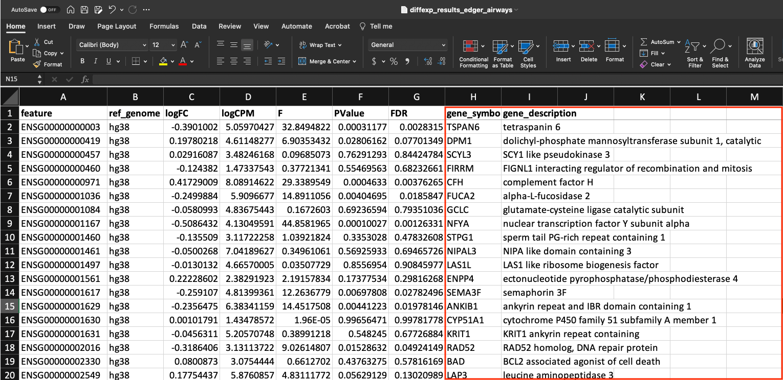
Our differential expression results look like this:
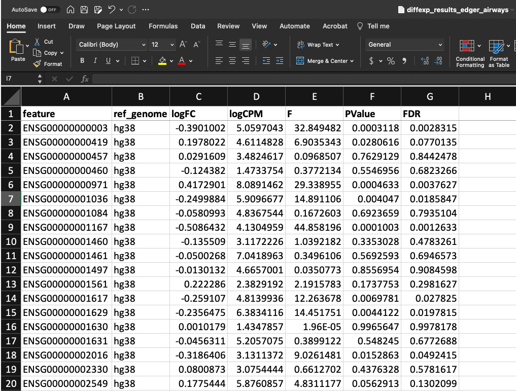
In the first column, we have our genes as Ensembl IDs followed by a column describing the reference genome used and then our differential expression results (logFC, logCPM, F, PValue, FDR).
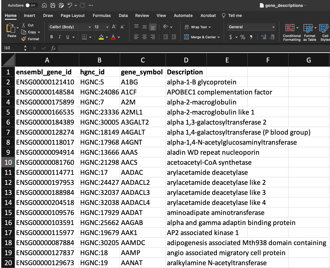
We would like to combine this information with the official gene symbols and their descriptions from HGNC. That data looks like this:
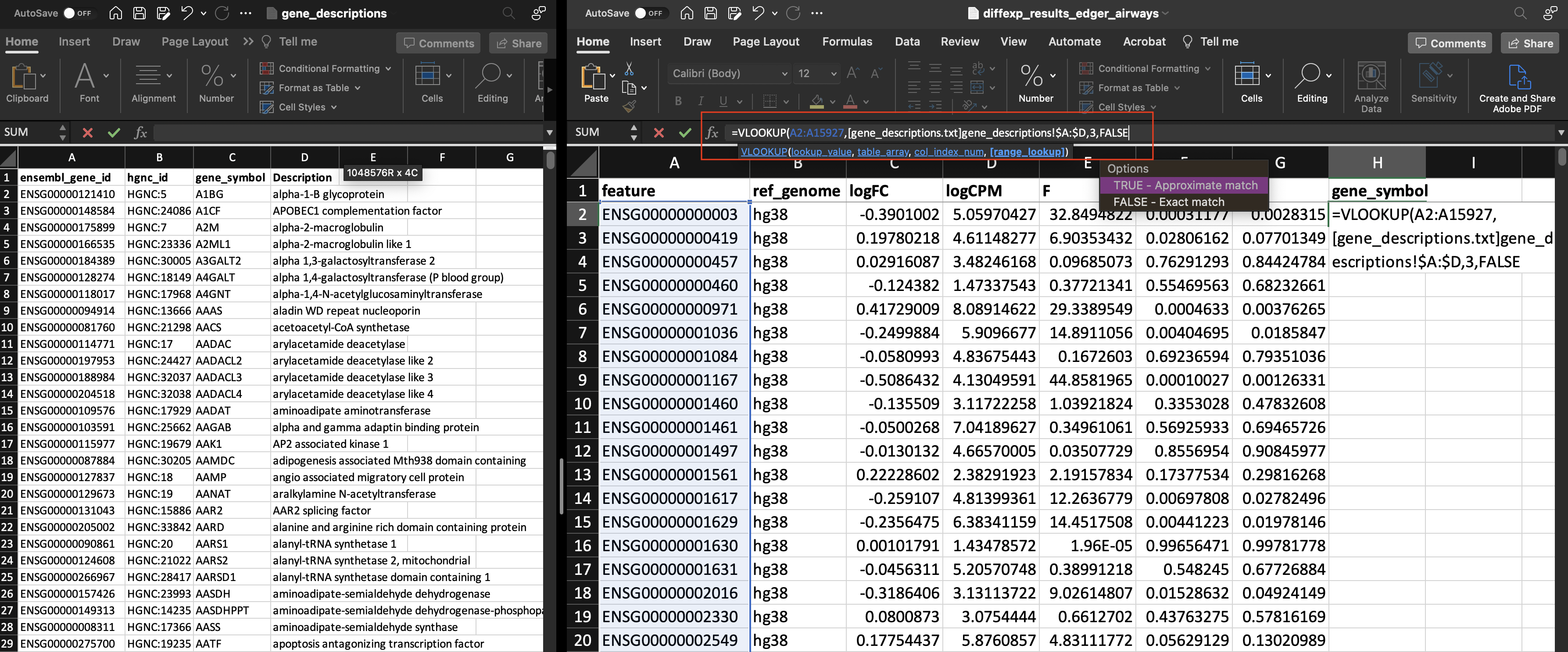
Let's add gene_symbol and Description to our differential expression results.
We have to add these columns one at a time, so we will begin with gene_symbol.
Using the VLOOKUP function (=VLOOKUP), we will enter the following 4 components:
lookup_value: (A2:A15927)table_array: Here we are selecting a range of columns and rows from a different file ([gene_descriptions.txt]gene_descriptions!\$A:\$D)col_index_num: (3)range_lookup(FALSE)
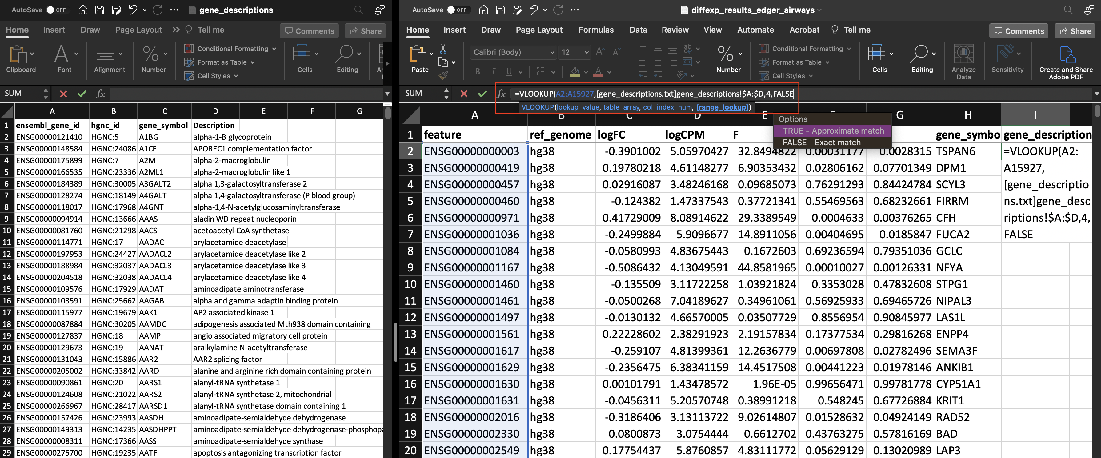
Now, let's add our gene_description.
lookup_value: (A2:A15927)table_array: Here we are selecting a range of columns and rows from a different file ([gene_descriptions.txt]gene_descriptions!\$A:\$D)col_index_num: (4)range_lookup(FALSE)
Notice the only thing that changed in our VLOOKUP formula was the col_index_num.
And our final result:
This was pretty easy with excel and required minimal wrangling. We will see an example at the end of this lesson where the opposite is true. But first, let's see how we can get the same result with R.
VLOOKUP with R: combining gene expression results with gene symbols and descriptions
What is R?
R is a language and environment for statistical computing and graphics. ---r-project.org.
- Open-source and widely used by scientists, not just bioinformaticians.
- Extensible. R functionality is greatly expanded by using packages created by the R community.
- Maintained by a network of collaborators - The R Core Team
- A resource for and by scientists
- R functionality makes it easy to develop and share packages on any topic.
Why use R?
R is a particularly great resource for statistical analysis, plotting, and report generating.
It's wide use translates to functions and packages covering a broad range of topics.
- CRAN has 18,000 + packages.
- Bioconductor (v 3.16) includes 2,183 software packages, 416 experiment data packages, 909 annotation packages, 28 workflows, and 8 books.
Help is easy to find with a quick web search.
R allows for reproducibility!
Why not use R?
The primary reason not to use R is that it has a rather steep learning curve. The best way to learn R is to use R, but to use R, you need to learn a bit of R.
Gene Expression Example.
We want to add the columns gene_symbol and Description from one data table to another data table containing our differential expression results.
First, let's load our data.
gene_info_fp<-file.path("..","data","S1_VLOOKUP","gene_expression",
              "gene_descriptions.txt")

dexp_fp<-file.path("..","data","S1_VLOOKUP","gene_expression",
                   "diffexp_results_edger_airways.txt")

gene_info<-read.delim(gene_info_fp)

dexp<-read.delim(dexp_fp)
There are several ways to do this in R.
Approach 1: Using base R merge()
Without installing any other packages we can use the base R function merge, which will "merge two data frames by common columns or row names, or do other versions of database join operations."
mdf<-merge(gene_info[c(1,3,4)],dexp,by.x="ensembl_gene_id",
           by.y="feature",all.y=TRUE)

#Creating a tibble simply to limit the viewable output
tibble::as_tibble(mdf)
# A tibble: 15,926 × 9
   ensembl_gene_id gene_symbol Description     ref_genome   logFC logCPM       F
   <chr>           <chr>       <chr>           <chr>        <dbl>  <dbl>   <dbl>
 1 ENSG00000000003 TSPAN6      tetraspanin 6   hg38       -0.390    5.06 32.8
 2 ENSG00000000419 DPM1        dolichyl-phosp… hg38        0.198    4.61  6.90
 3 ENSG00000000457 SCYL3       SCY1 like pseu… hg38        0.0292   3.48  0.0969
 4 ENSG00000000460 FIRRM       FIGNL1 interac… hg38       -0.124    1.47  0.377
 5 ENSG00000000971 CFH         complement fac… hg38        0.417    8.09 29.3
 6 ENSG00000001036 FUCA2       alpha-L-fucosi… hg38       -0.250    5.91 14.9
 7 ENSG00000001084 GCLC        glutamate-cyst… hg38       -0.0581   4.84  0.167
 8 ENSG00000001167 NFYA        nuclear transc… hg38       -0.509    4.13 44.9
 9 ENSG00000001460 STPG1       sperm tail PG-… hg38       -0.136    3.12  1.04
10 ENSG00000001461 NIPAL3      NIPA like doma… hg38       -0.0500   7.04  0.350
# … with 15,916 more rows, and 2 more variables: PValue <dbl>, FDR <dbl>
Approach 2: using join functions from dplyr
In this case, we are going to use a left_join in order to retain all rows in our differential expression results. If we only wanted to include matching values, we could instead use an inner_join. See the documentation here.
A left_join keeps all observations in x (the first argument).
It's worth exploring the different types of joins in detail, as these can be extremely useful for controlling data frame merges. See mutating joins and filtering joins from dplyr.
library(dplyr)
Attaching package: 'dplyr'
The following objects are masked from 'package:stats':

    filter, lag
The following objects are masked from 'package:base':

    intersect, setdiff, setequal, union
ljdf<-left_join(dexp, gene_info[c(1,3,4)],
                by = c("feature" = "ensembl_gene_id"))

#Reordered for aesthetics only
tibble::as_tibble(select(ljdf,1,8:9,2:7))
# A tibble: 15,926 × 9
   feature     gene_symbol Description ref_genome   logFC logCPM       F  PValue
   <chr>       <chr>       <chr>       <chr>        <dbl>  <dbl>   <dbl>   <dbl>
 1 ENSG000000… TSPAN6      tetraspani… hg38       -0.390    5.06 32.8    3.12e-4
 2 ENSG000000… DPM1        dolichyl-p… hg38        0.198    4.61  6.90   2.81e-2
 3 ENSG000000… SCYL3       SCY1 like … hg38        0.0292   3.48  0.0969 7.63e-1
 4 ENSG000000… FIRRM       FIGNL1 int… hg38       -0.124    1.47  0.377  5.55e-1
 5 ENSG000000… CFH         complement… hg38        0.417    8.09 29.3    4.63e-4
 6 ENSG000000… FUCA2       alpha-L-fu… hg38       -0.250    5.91 14.9    4.05e-3
 7 ENSG000000… GCLC        glutamate-… hg38       -0.0581   4.84  0.167  6.92e-1
 8 ENSG000000… NFYA        nuclear tr… hg38       -0.509    4.13 44.9    1.00e-4
 9 ENSG000000… STPG1       sperm tail… hg38       -0.136    3.12  1.04   3.35e-1
10 ENSG000000… NIPAL3      NIPA like … hg38       -0.0500   7.04  0.350  5.69e-1
# … with 15,916 more rows, and 1 more variable: FDR <dbl>
Note
There are also packages with specific VLOOKUP functions, but many of these are using match and merge under the hood. For example, check out lookup.
Example 2: Understanding 10X TCR data using annotation output from the cellranger vdj pipeline.
Load the data:
library(readxl)

TCR_fp<-file.path("..","data","S1_VLOOKUP","TCR_example",
              "4261-R1_filtered_contig_annotations.xlsx")


df<-read_excel(TCR_fp)

knTCR<-read_excel(TCR_fp,sheet=2)
Here, we want to use annotation data from a 10X TCR sequencing run and compare known TCR sequences. Specifically, we want to answer several questions using the contig annotation files from the cellranger vdj pipeline. For a detailed description of each column, see "Contig annotation CSV files", here.
Here's a summary of the cellranger vdj annotation file:
glimpse(df)
Rows: 8,028
Columns: 31
$ barcode               <chr> "AAACCTGAGGCGATAC-1", "AAACCTGAGGCGATAC-1", "AAA…
$ is_cell               <lgl> TRUE, TRUE, TRUE, TRUE, TRUE, TRUE, TRUE, TRUE, …
$ contig_id             <chr> "AAACCTGAGGCGATAC-1_contig_1", "AAACCTGAGGCGATAC…
$ high_confidence       <lgl> TRUE, TRUE, TRUE, TRUE, TRUE, TRUE, TRUE, TRUE, …
$ length                <dbl> 483, 519, 518, 483, 589, 507, 483, 568, 574, 490…
$ chain                 <chr> "TRB", "TRA", "TRA", "TRB", "TRA", "TRB", "TRB",…
$ v_gene                <chr> "TRBV4-1*01", "TRAV35*01", "TRAV35*01", "TRBV4-1…
$ d_gene                <chr> NA, NA, NA, NA, NA, NA, NA, NA, NA, NA, NA, NA, …
$ j_gene                <chr> "TRBJ2-1*01", "TRAJ28*01", "TRAJ28*01", "TRBJ2-1…
$ c_gene                <chr> "TRBC2*01", "TRAC*01", "TRAC*01", "TRBC2*01", "T…
$ full_length           <lgl> TRUE, TRUE, TRUE, TRUE, TRUE, TRUE, TRUE, TRUE, …
$ productive            <lgl> TRUE, TRUE, TRUE, TRUE, TRUE, TRUE, TRUE, TRUE, …
$ fwr1                  <chr> "DTEVTQTPKHLVMGMTNKKSLKCEQH", "GQQLNQSPQSMFIQEGE…
$ fwr1_nt               <chr> "GACACTGAAGTTACCCAGACACCAAAACACCTGGTCATGGGAATGAC…
$ cdr1                  <chr> "MGHRA", "SIFNT", "SIFNT", "MGHRA", "TSINN", "SG…
$ cdr1_nt               <chr> "ATGGGGCACAGGGCT", "AGCATATTTAACACC", "AGCATATTT…
$ fwr2                  <chr> "MYWYKQKAKKPPELMFV", "WLWYKQDPGEGPVLLIA", "WLWYK…
$ fwr2_nt               <chr> "ATGTATTGGTACAAGCAGAAAGCTAAGAAGCCACCGGAGCTCATGTT…
$ cdr2                  <chr> "YSYEKL", "LYKAGEL", "LYKAGEL", "YSYEKL", "IRSNE…
$ cdr2_nt               <chr> "TACAGCTATGAGAAACTC", "TTATATAAGGCTGGTGAATTG", "…
$ fwr3                  <chr> "SINESVPSRFSPECPNSSLLNLHLHALQPEDSALYL", "TSNGRLT…
$ fwr3_nt               <chr> "TCTATAAATGAAAGTGTGCCAAGTCGCTTCTCACCTGAATGCCCCAA…
$ cdr3                  <chr> "CASSQALAGPEQFF", "CAGQLISGAGSYQLTF", "CAGQLISGA…
$ cdr3_nt               <chr> "TGCGCCAGCAGCCAAGCACTAGCGGGTCCAGAGCAGTTCTTC", "T…
$ fwr4                  <chr> "GPGTRLTVL", "GKGTKLSVIP", "GKGTKLSVIP", "GPGTRL…
$ fwr4_nt               <chr> "GGGCCAGGGACACGGCTCACCGTGCTAG", "GGGAAGGGGACCAAA…
$ reads                 <dbl> 11975, 773, 1178, 9780, 2375, 16987, 886, 19290,…
$ umis                  <dbl> 78, 5, 8, 57, 18, 119, 5, 140, 64, 9, 40, 32, 44…
$ raw_clonotype_id      <chr> "clonotype1", "clonotype1", "clonotype1", "clono…
$ raw_consensus_id      <chr> "clonotype1_consensus_1", "clonotype1_consensus_…
$ exact_subclonotype_id <dbl> 3, 3, 3, 3, 1, 1, 1, 1, 1, 1, 1, 1, 1, 1, 3, 3, …
Here is what our known TCR data frame looks like:
knTCR
# A tibble: 8 × 6
  Tumor Neoantigen CDR3b             TRBV        CDR3a            TRAV
  <dbl> <chr>      <chr>             <chr>       <chr>            <chr>
1  4261 ATL2.1     CASSLAPQGEAFF     TRBV7-6*01  CAGHGGATNKLIF    TRAV35*01
2  4261 ATL2.2     CASSQERGLAGFNEQFF TRBV4-1*01  CASYTNAGKSTF     TRAV24*01
3  4261 ATL2.3     CASSQALAGPEQFF    TRBV4-1*01  CAGQLISGAGSYQLTF TRAV35*01
4  4261 GATA6.1    CASSFEADTQYF      TRBV12-4*01 CAMSSYSSASKIIF   TRAV12-3*01
5  4261 GATA6.2    CATSLEADTQYF      TRBV12-4*01 CAMSSYSSASKIIF   TRAV12-3*01
6  4261 GATA6.3    CASSLYGPLSSYNEQFF TRBV12-4*01 CILSGGGSNYKLTF   TRAV26-2*01
7  4261 GATA6.4    CASSLEATSVYNEQFF  TRBV5-4*01  CILRENNARLMF     TRAV26-2*01
8  4261 GATA6.5    CASSIDGAGGPPGELFF TRBV19*01   CASRTDSWGKLQF    TRAV38-1*01
We want to start by answering a few questions:
How often do the TCRs in knTCR show up in the cellranger output? (Counts)
How often do the CDR3a sequences match; how often do the CDR3b sequences match, and how often do we see that both match together?
In addition to counts, we want to actually be able to examine matched content.
Using Excel
These questions can be answered in excel. However, the data would need to be reshaped. To see what I mean, let's take a brief look at the data in Excel.
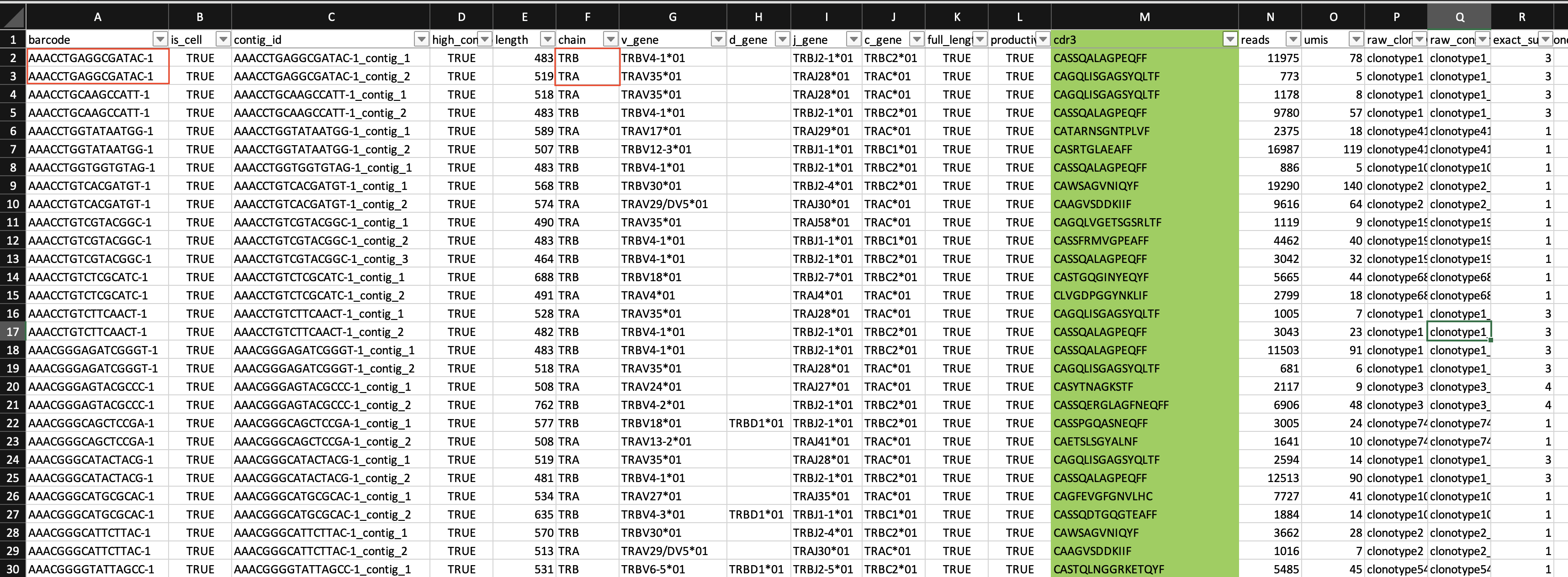
Notice that there are two or more rows represented by a single cell barcode, and each row is associated with TCR alpha chain or beta chain data. While most cells have a single TRA or TRB sequence, some have two TRAs or two TRBs. These will likely need to be assessed for potential error.
If we want to match CDR3a and CDR3b sequences simultaneously, ideally these should be in the same row.
Let's check out our standard VLOOKUP, without any data reshaping.
We will create two new columns in our data named "knTRA_match" and "knTRB_match".
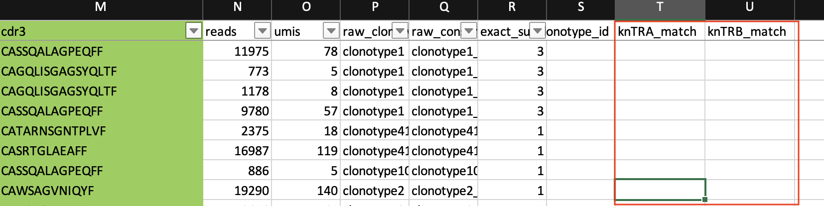
Now, let's do a vlookup to match the cdr3 sequences.
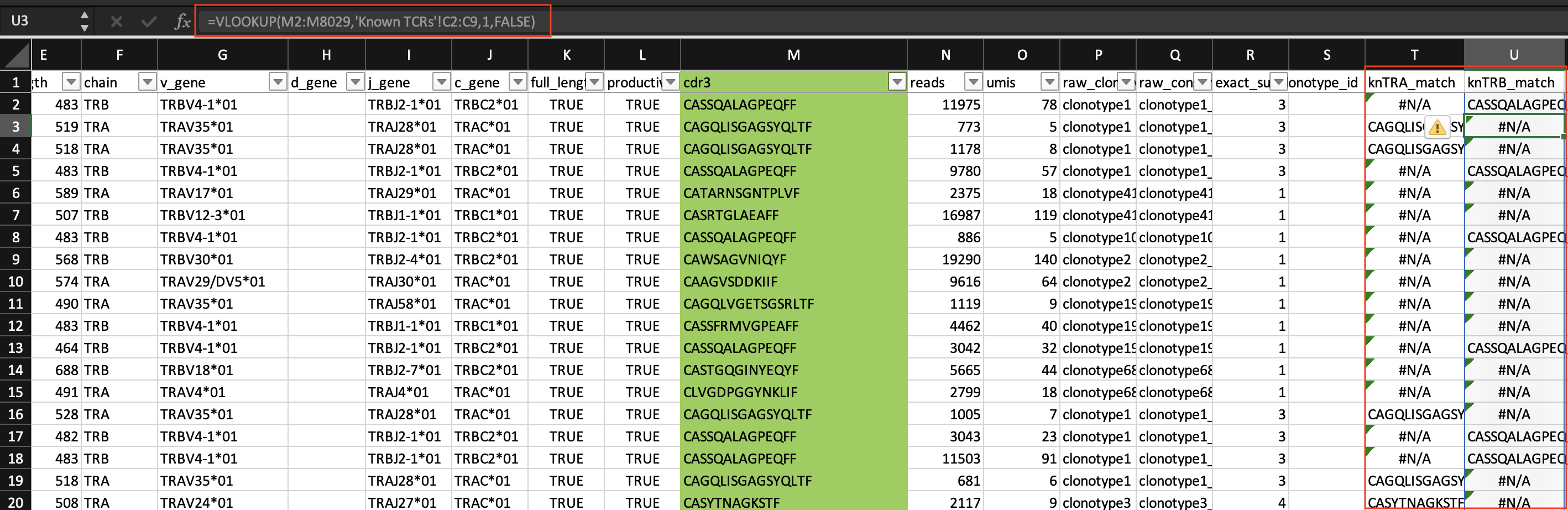
This output is pretty rough without doing additional Excel wizardry for data reshaping. This data set isn't small (8,028 rows by 34 columns), so the probability of making a mistake while reformatting the data is high. Also, it isn't easy to trace steps in Excel, so if I plan to repeat this type of analysis in the future, I will likely spend a similar amount of time completing this task.
Tip
Using R will make this analysis less error prone and more reproducible. Once we generate a script, we can refer back to it and hopefully make minimal edits or no edits at all to apply the same steps to a new data set.
Return to R
Let's reshape the data. I will rely heavily on dplyr functions to perform these tasks.
First, I want to isolate the alpha chain and beta chain data.
#isolate alpha and beta
dfTRA<-df %>% filter(chain=="TRA")
colnames(dfTRA)<-paste(colnames(dfTRA),"TRA", sep="_")
dfTRB<-df %>% filter(chain=="TRB")
colnames(dfTRB)<-paste(colnames(dfTRB),"TRB", sep="_")
I'm also going to modify the column names in knTCR just to make my life easier for joining data sets later.
#modify column names in knTCR for easier matching
colnames(knTCR)
[1] "Tumor"      "Neoantigen" "CDR3b"      "TRBV"       "CDR3a"
[6] "TRAV"
colnames(knTCR)<-c("Tumor","Neoantigen","cdr3_TRB",
                   "v_gene_TRB","cdr3_TRA",
                   "v_gene_TRA")
Next, I'm going to join the data back together using a full_join. A full_join keeps all observations from both datasets.
#Join filtered data frames
df_full<-full_join(dfTRA,dfTRB,by = c("barcode_TRA" = "barcode_TRB")) %>%
  select(barcode_TRA,v_gene_TRA,cdr3_TRA,reads_TRA,
         raw_clonotype_id_TRA,v_gene_TRB,cdr3_TRB,
         reads_TRB,raw_clonotype_id_TRB)
#change name of first column to just barcode
colnames(df_full)[1]<-"barcode"

#Add a column with unique identifier
df_full$identifier<-1:nrow(df_full)

df_full
# A tibble: 4,649 × 10
   barcode    v_gene_TRA cdr3_TRA reads_TRA raw_clonotype_i… v_gene_TRB cdr3_TRB
   <chr>      <chr>      <chr>        <dbl> <chr>            <chr>      <chr>
 1 AAACCTGAG… TRAV35*01  CAGQLIS…       773 clonotype1       TRBV4-1*01 CASSQAL…
 2 AAACCTGCA… TRAV35*01  CAGQLIS…      1178 clonotype1       TRBV4-1*01 CASSQAL…
 3 AAACCTGGT… TRAV17*01  CATARNS…      2375 clonotype415     TRBV12-3*… CASRTGL…
 4 AAACCTGTC… TRAV29/DV… CAAGVSD…      9616 clonotype2       TRBV30*01  CAWSAGV…
 5 AAACCTGTC… TRAV35*01  CAGQLVG…      1119 clonotype19      TRBV4-1*01 CASSFRM…
 6 AAACCTGTC… TRAV35*01  CAGQLVG…      1119 clonotype19      TRBV4-1*01 CASSQAL…
 7 AAACCTGTC… TRAV4*01   CLVGDPG…      2799 clonotype684     TRBV18*01  CASTGQG…
 8 AAACCTGTC… TRAV35*01  CAGQLIS…      1005 clonotype1       TRBV4-1*01 CASSQAL…
 9 AAACGGGAG… TRAV35*01  CAGQLIS…       681 clonotype1       TRBV4-1*01 CASSQAL…
10 AAACGGGAG… TRAV24*01  CASYTNA…      2117 clonotype3       TRBV4-2*01 CASSQER…
# … with 4,639 more rows, and 3 more variables: reads_TRB <dbl>,
#   raw_clonotype_id_TRB <chr>, identifier <int>
Now for matching and counting where our knowns are found in our unknowns.
Let's start with matching all combinations of cdr3_TRA and cdr3_TRB.
#create a data frame and inner join with knTCR
fullTRATCR<-knTCR %>% select(cdr3_TRA,cdr3_TRB) %>%
  distinct(cdr3_TRA,cdr3_TRB) %>%
  inner_join(df_full)
Joining, by = c("cdr3_TRA", "cdr3_TRB")
An inner_join() only keeps observations from x that have a matching key in y.
The most important property of an inner join is that unmatched rows in either input are not included in the result. This means that generally inner joins are not appropriate in most analyses, because it is too easy to lose observations.---dplyr.tidyverse.org
#Count where we have matches
fullTRATCRc<- fullTRATCR %>%
  count(cdr3_TRA,cdr3_TRB,name="TRATRB_match_count")
Next, we can examine unique matches of cdr3_TRA only. However, we want to avoid double counting duplicate cdr3_TRAs as an artifact of data reshaping. To do this, we are going to create a data frame to use for filtering. We will do the same thing for TRB.
#create a table to avoid double counting

#we are only examining cells that had a match for both TRA and TRB
#cdr3 sequences.
filttab_TRA<-df_full %>% filter(barcode %in% fullTRATCR$barcode) %>%
  group_by(barcode) %>%
  #count number of barcodes and number of distinct TRA or TRB
  summarize(n_barcode=n(),n_distinct_TRA=n_distinct(cdr3_TRA),
            n_distinct_TRB=n_distinct(cdr3_TRB)) %>%
  #We want to be able to filter any instances of two barcodes where the
  #TRA is the same
  filter(n_barcode==2 & n_distinct_TRA==1)

#repeat for TRB
filttab_TRB<-df_full %>% filter(barcode %in% fullTRATCR$barcode) %>%
  group_by(barcode) %>%
  summarize(n_barcode=n(),n_distinct_TRA=n_distinct(cdr3_TRA),
            n_distinct_TRB=n_distinct(cdr3_TRB)) %>%
  filter(n_barcode==2 & n_distinct_TRB==1)
Get unique matches of cdr3_TRA.
#to look at unique matches, we will anti-join to drop
#previously matched rows
a<-df_full %>% anti_join(fullTRATCR) %>%
  #filter out the barcodes from our filter table above
  filter(!barcode %in% filttab_TRA$barcode) %>%
  group_by(barcode) %>%
  #only count unique cdr3_TRA per barcode
  distinct(cdr3_TRA,.keep_all=TRUE) %>% ungroup() %>%
  #perform an inner_join to match with knTCR
  inner_join(x=distinct(select(knTCR,cdr3_TRA)),y=.)
Joining, by = c("barcode", "v_gene_TRA", "cdr3_TRA", "reads_TRA",
"raw_clonotype_id_TRA", "v_gene_TRB", "cdr3_TRB", "reads_TRB",
"raw_clonotype_id_TRB", "identifier")
Joining, by = "cdr3_TRA"
#retrieve match counts
ac<-a %>% count(cdr3_TRA,name="TRA_match_count")

ac
# A tibble: 4 × 2
  cdr3_TRA         TRA_match_count
  <chr>                      <int>
1 CAGQLISGAGSYQLTF               6
2 CAMSSYSSASKIIF                 5
3 CASYTNAGKSTF                  29
4 CILSGGGSNYKLTF                 2
Get unique matches of cdr3_TRB.
b<-df_full %>% anti_join(fullTRATCR) %>%
  filter(!barcode %in% filttab_TRB$barcode) %>%
  group_by(barcode) %>%
  distinct(cdr3_TRB,.keep_all=TRUE) %>% ungroup() %>%
  inner_join(x=distinct(select(knTCR,cdr3_TRB)),y=.)
Joining, by = c("barcode", "v_gene_TRA", "cdr3_TRA", "reads_TRA",
"raw_clonotype_id_TRA", "v_gene_TRB", "cdr3_TRB", "reads_TRB",
"raw_clonotype_id_TRB", "identifier")
Joining, by = "cdr3_TRB"
bc <- b %>% count(cdr3_TRB,name="TRB_match_count")

bc
# A tibble: 5 × 2
  cdr3_TRB          TRB_match_count
  <chr>                       <int>
1 CASSFEADTQYF                   27
2 CASSIDGAGGPPGELFF               1
3 CASSLYGPLSSYNEQFF              73
4 CASSQALAGPEQFF                 96
5 CASSQERGLAGFNEQFF              74
Now, let's create a table of match counts.
ctab<-knTCR %>%
  left_join(ac) %>%
  left_join(bc) %>%
  left_join(fullTRATCRc) %>%
  #This replaces NAs with 0.
  mutate(across(where(is.numeric),~ifelse(is.na(.),0,.)))
Joining, by = "cdr3_TRA"
Joining, by = "cdr3_TRB"
Joining, by = c("cdr3_TRB", "cdr3_TRA")
ctab
# A tibble: 8 × 9
  Tumor Neoantigen cdr3_TRB       v_gene_TRB cdr3_TRA v_gene_TRA TRA_match_count
  <dbl> <chr>      <chr>          <chr>      <chr>    <chr>                <dbl>
1  4261 ATL2.1     CASSLAPQGEAFF  TRBV7-6*01 CAGHGGA… TRAV35*01                0
2  4261 ATL2.2     CASSQERGLAGFN… TRBV4-1*01 CASYTNA… TRAV24*01               29
3  4261 ATL2.3     CASSQALAGPEQFF TRBV4-1*01 CAGQLIS… TRAV35*01                6
4  4261 GATA6.1    CASSFEADTQYF   TRBV12-4*… CAMSSYS… TRAV12-3*…               5
5  4261 GATA6.2    CATSLEADTQYF   TRBV12-4*… CAMSSYS… TRAV12-3*…               5
6  4261 GATA6.3    CASSLYGPLSSYN… TRBV12-4*… CILSGGG… TRAV26-2*…               2
7  4261 GATA6.4    CASSLEATSVYNE… TRBV5-4*01 CILRENN… TRAV26-2*…               0
8  4261 GATA6.5    CASSIDGAGGPPG… TRBV19*01  CASRTDS… TRAV38-1*…               0
# … with 2 more variables: TRB_match_count <dbl>, TRATRB_match_count <dbl>
Lastly, we may want to examine where we had matches.
Note
You will need to install the package data.table to use rbindlist.
tables<-list(a,b,fullTRATCR)
names(tables)<-c("TRA","TRB","TRA_TRB")
matches<-data.table::rbindlist(tables,use.names=TRUE,idcol="Type_of_Match")
df_full2<-df_full %>% left_join(matches)
Joining, by = c("barcode", "v_gene_TRA", "cdr3_TRA", "reads_TRA",
"raw_clonotype_id_TRA", "v_gene_TRB", "cdr3_TRB", "reads_TRB",
"raw_clonotype_id_TRB", "identifier")
df_full2
# A tibble: 4,649 × 11
   barcode    v_gene_TRA cdr3_TRA reads_TRA raw_clonotype_i… v_gene_TRB cdr3_TRB
   <chr>      <chr>      <chr>        <dbl> <chr>            <chr>      <chr>
 1 AAACCTGAG… TRAV35*01  CAGQLIS…       773 clonotype1       TRBV4-1*01 CASSQAL…
 2 AAACCTGCA… TRAV35*01  CAGQLIS…      1178 clonotype1       TRBV4-1*01 CASSQAL…
 3 AAACCTGGT… TRAV17*01  CATARNS…      2375 clonotype415     TRBV12-3*… CASRTGL…
 4 AAACCTGTC… TRAV29/DV… CAAGVSD…      9616 clonotype2       TRBV30*01  CAWSAGV…
 5 AAACCTGTC… TRAV35*01  CAGQLVG…      1119 clonotype19      TRBV4-1*01 CASSFRM…
 6 AAACCTGTC… TRAV35*01  CAGQLVG…      1119 clonotype19      TRBV4-1*01 CASSQAL…
 7 AAACCTGTC… TRAV4*01   CLVGDPG…      2799 clonotype684     TRBV18*01  CASTGQG…
 8 AAACCTGTC… TRAV35*01  CAGQLIS…      1005 clonotype1       TRBV4-1*01 CASSQAL…
 9 AAACGGGAG… TRAV35*01  CAGQLIS…       681 clonotype1       TRBV4-1*01 CASSQAL…
10 AAACGGGAG… TRAV24*01  CASYTNA…      2117 clonotype3       TRBV4-2*01 CASSQER…
# … with 4,639 more rows, and 4 more variables: reads_TRB <dbl>,
#   raw_clonotype_id_TRB <chr>, identifier <int>, Type_of_Match <chr>
Now that we have this code, we can use it to examine additional cellranger vdj annotation output files. We would just need to make sure that the column names of any known TCR data we are interested in comparing are the same.
Interested in learning R
Check out our introductory courses:
References
Acknowledgements
The 10X TCR example data was generously provided by Paul Robbins. The differential expression results were derived from data extracted from the R package, airway, from Himes et al. 2014.
What's next for the BTEP Coding Club?
April 19th, 2023: Join us for a demo on Jupyter notebooks by Joe Wu.