ComplexHeatmap and Enhanced Volcano
Learning Objectives
This Coding Club will focus on heatmaps and volcano plots. At the end of this session, participants will be able to
-
Describe two examples of when a heatmap can be used in genomic data analysis.
-
Provide rationale for scaling data before generating a heatmap and the method used for scaling.
-
Construct and customize a heatmap using the package ComplexHeatmap.
-
Describe a volcano plot and create one using the package EnhancedVolcano.
## Store input data directory as data_path
data_path <- "~/onedrive/GAU/BTEP/BTEP_Coding_Club/data/S6_ComplexHeatmapEnhancedVolcano"
Heatmap
Background on heatmap
A heatmap represents numerical data on a color scale and is often combined with a dendrogram to facilitate visualization of clusters and to identify patterns among study variables. For instance, they can be used to visualize gene expression data (Figure 1) and correlation among samples during quality check in genomic data analysis (Figure 2).
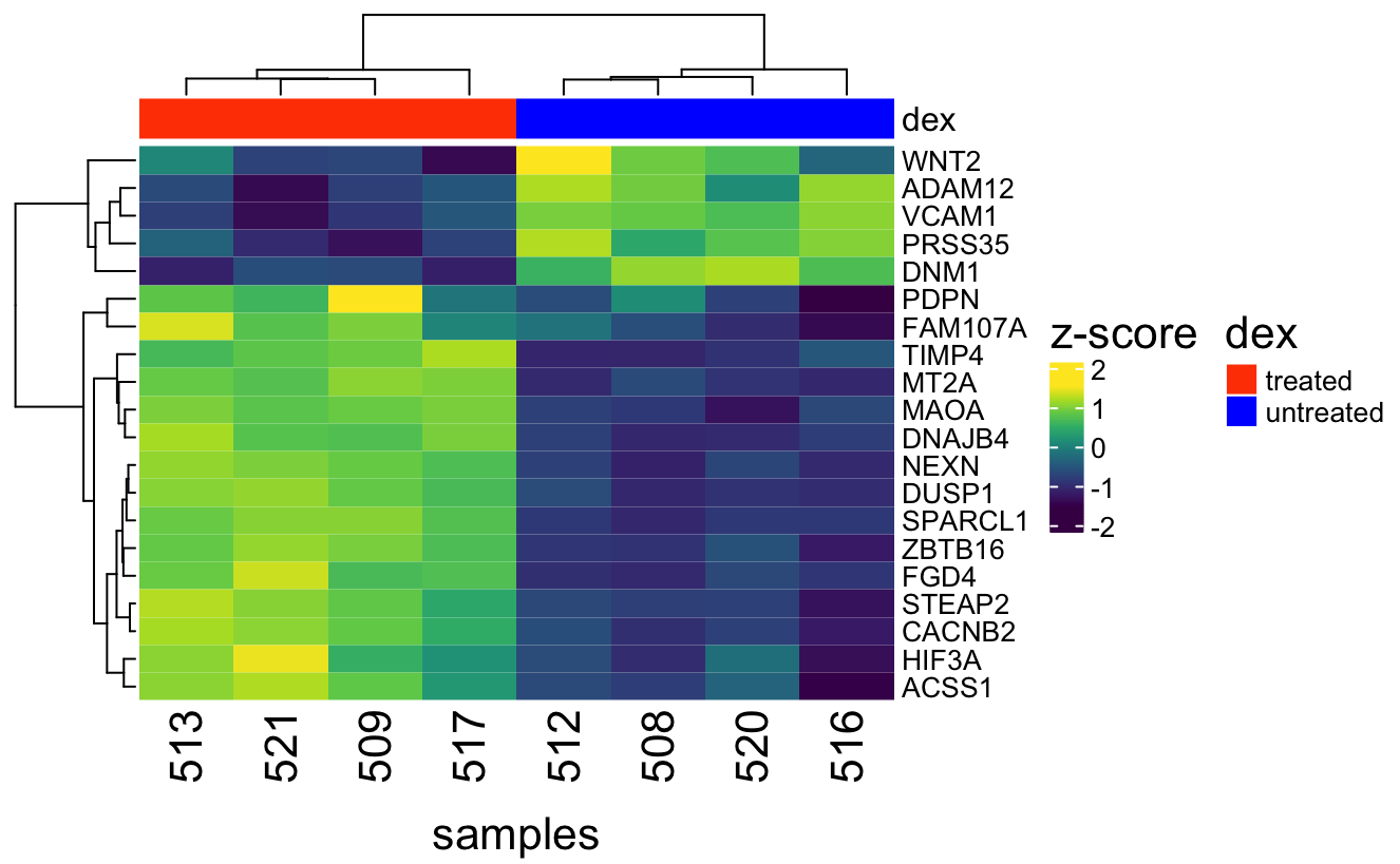
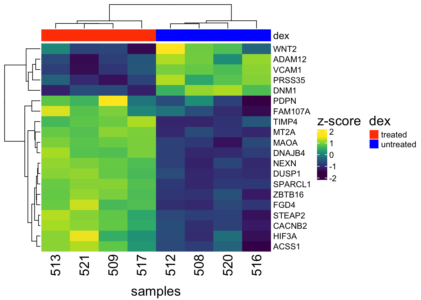
Figure 1: Heatmap and dendrogram of the top 20 differential expressed genes from the Airway study reveals distinct gene expression patterns between dexamethasone treated and untreated cells.
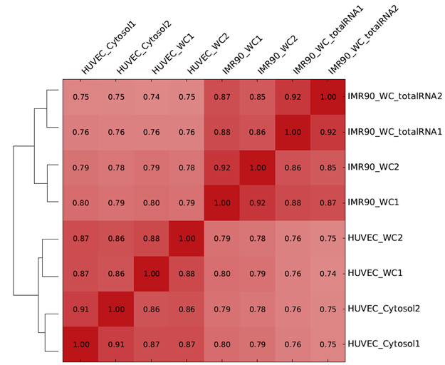
Figure 2: Heatmap and dendrogram showing sample correlation in an RNA sequecing experiment (source: deepTools), which is used as a quality check tool. It is expected that samples within the same treatment group cluster together and are more correlated with each other.
Step-by-step guide to making a heatmap
Step 1: Import the data
This exercise will use the package ComplexHeatmap and the normalized (log2 counts per million or log2 CPM) count values from the top 20 differential expressed genes from the Airway study to reproduce Figure 1. This data is housed in the file RNAseq_mat_top20.csv and the steps below will be followed to import it into the R work space.
-
Use
paste0to construct the full path to RNAseq_mat_top20.csv, which is composed the data_path object, a "/", and the file name. This path will be stored as my_file. -
Import the data set using
read.csvusing my_file as the argument with the options below.-
Set column 1 (ie. genes) as the row name.
-
Set
check.names=FALSEto skip checking on column header format. -
Store data as counts_df.
-
my_file <- paste0(data_path,"/","RNAseq_mat_top20.csv")
counts_df <- read.csv(my_file,row.names=1,check.names=FALSE)
The counts_df table contains only expression counts for the top 20 differential expressed genes. This is done to avoid cluttering the heatmap. In this dataset, genes are listed as row names and column headings represent sample identifiers. The Airway study profiled the transcriptome of several airway smooth muscle cell lines under either control or dexamethasone treated conditions. Samples 508, 512, 516, and 520 are control while 509, 513, 517, and 521 were treated with dexamethasone.
counts_df
               508      509        512      513        516        517
WNT2     4.6945537 1.332858  5.9837204 2.898648  2.1105784 -0.1655252
DNM1     6.1807353 4.441965  5.6600240 3.981513  5.8002923  3.9603755
ZBTB16  -1.8635225 5.257967 -1.7771519 4.902223 -2.9319722  4.2830866
DUSP1    4.9365511 8.019074  5.6075681 8.302196  5.0283417  7.7229898
HIF3A    1.0139913 3.374457  1.5752503 4.154740  0.4928878  2.8335879
MT2A     6.2485140 8.276988  5.7828554 8.070846  5.7583897  8.2015855
FGD4     4.1324133 6.239578  4.2162202 6.502058  4.3127101  6.3038216
PRSS35   3.9300156 1.143441  5.1890727 2.649826  4.8483066  2.0681419
ADAM12   6.6778583 4.822508  6.9845104 4.964557  6.8603125  5.1089646
SPARCL1  1.5547097 6.720696  2.0225956 6.349355  2.0283400  6.0058626
ACSS1    3.7148373 5.565503  3.8693768 5.799204  2.9163018  4.8879038
TIMP4    0.5987937 3.768203  0.5805233 3.375168  1.5275170  4.2531196
STEAP2   5.9092730 7.723250  6.0463677 8.154854  5.3438076  7.2693880
PDPN     5.3575325 7.206776  4.3556272 6.283956  3.1219541  5.0257422
NEXN     6.3863354 8.609984  6.7947534 8.834731  6.4735995  8.4246611
DNAJB4   5.0327684 6.508720  5.2842361 6.874350  5.2410589  6.7002033
VCAM1    5.3942205 1.719779  5.5824203 1.968348  5.7626351  2.5346502
CACNB2   1.9123342 5.242302  2.5823040 5.836526  1.4870379  4.5812252
FAM107A -0.6391149 3.832389  0.5805233 4.974158 -2.9319722  1.1757099
MAOA     4.3461550 7.581819  4.5336120 7.751647  4.7078611  7.7347841
               520       521
WNT2     4.2828513 1.2370000
DNM1     6.2853003 4.4889554
ZBTB16  -0.5150407 5.7791730
DUSP1    5.1432459 8.3967093
HIF3A    2.2501244 4.7905809
MT2A     5.9163628 7.9334918
FGD4     4.5898185 7.0390817
PRSS35   4.4826222 1.6072514
ADAM12   5.8173287 4.1437775
SPARCL1  2.0348850 6.7198328
ACSS1    4.2331375 5.9951083
TIMP4    0.8195520 3.6386792
STEAP2   5.9403923 7.9302905
PDPN     4.1896911 5.9928782
NEXN     6.8533406 8.7188968
DNAJB4   5.0601499 6.5413581
VCAM1    5.0380493 0.6943811
CACNB2   2.3103727 5.6046874
FAM107A -1.7659813 3.2627622
MAOA     3.5365766 7.4238335
Step 2: Activate the ComplexHeatmap package
Load the ComplexHeatmap package using the library command.
library(ComplexHeatmap)
Step 3: Convert data frame to matrix
ComplexHeatmap takes matrices as input so counts_df will need to be converted into a matrix using as.matrix.
counts_matrix <- as.matrix(counts_df)
Step 4: Construct the heatmap
To construct the heatmap, use the Heatmap command. Note that the color scale bar takes on the title "matrix_1". This can be modified (shown later).
Heatmap(counts_matrix)

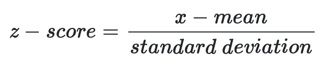
Scaling data by z score
An important step in generating a heatmap is to scale the data by z-score (see equation below). Given a vector of numbers, the z-score informs how many standard deviations is each number in the vector away from the mean of the numbers in that vector. For tabular data, z-score scaling can be applied to columns or rows, depending on which contains the dependent variable(s).
The mtcars data set, which is built into R helps to demonstrate the usefulness of scaling. To import a data set that is built into R, use the data command. Use as.matrix to convert the mtcars data into a matrix called car.
data(mtcars)
car <- as.matrix(mtcars)
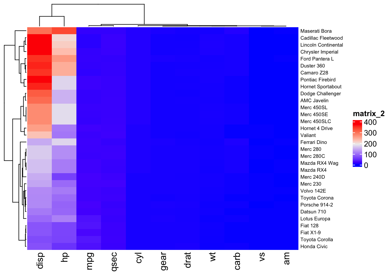
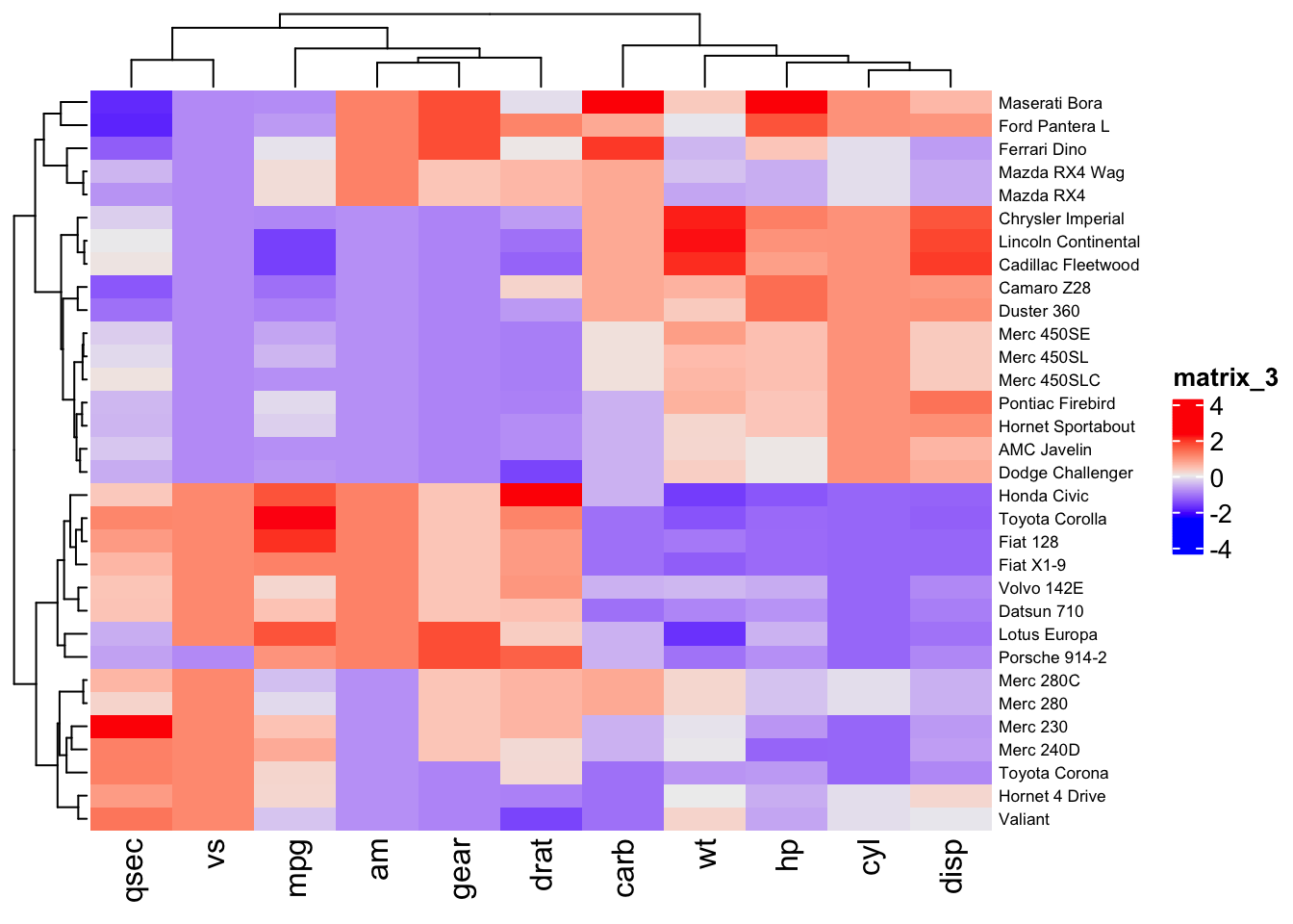
Below, the Heatmap command from ComplexHeatmap is used to generate a heatmap of the mtcars data set. The independent variables (car brands) are listed along the right vertical axis and attributes (dependent variables) of each car brand are listed along the bottom horizontal axis. The dependent variables "disp" and "hp" have large value ranges and hide differences in the other dependent variables, which have lower magnitude values. To correct this, scaling of the dependent variables is performed using R's scale function.
Note
In the Heatmap command below, the row_names_gp option is used to adjust the font size by setting it equal to gpar (short for graphical parameter). Within the parentheses following gpar, users can define fontsize.
Heatmap(car,row_names_gp=gpar(fontsize=6.5))
The scale function scales by column, which happens to be where the dependent variables for the mtcars dataset reside.
car_scaled <- scale(car)
The heatmap of the scaled mtcars data reveals differences in the attributes (or dependent variables) among the car brands. From the heatmap, it is clear that some car brands cluster together based on their attributes.
Heatmap(car_scaled,row_names_gp=gpar(fontsize=6.5))
Step 5: Scaling gene expression counts
The dependent variables (genes) in the expression counts matrix (counts_matrix) for the Airway data are listed as row identifiers. Thus, the transpose has to be taken using the t command prior to scaling using the scale command. After scaling, use the t command to transpose the scaled data so that column headers contain the samples identifiers and row identifiers contain genes.
counts_matrix_scaled <- t(counts_matrix)
counts_matrix_scaled <- scale(counts_matrix_scaled)
counts_matrix_scaled <- t(counts_matrix_scaled)
as.data.frame(counts_matrix_scaled)
               508        509        512         513        516         517
WNT2     0.9197709 -0.7095491  1.5445940  0.04934579 -0.3326097 -1.43577355
DNM1     1.1020538 -0.6708432  0.5711226 -1.14033280  0.7141439 -1.16188496
ZBTB16  -0.9399755  0.9696745 -0.9168150  0.87428063 -1.2264837  0.70825727
DUSP1   -1.0732608  0.8636752 -0.6516202  1.04157743 -1.0155832  0.67762735
HIF3A   -1.0235100  0.5384881 -0.6521063  1.05482754 -1.3683414  0.18057736
MT2A    -0.6534206  1.0565789 -1.0459700  0.88280180 -1.0665945  0.99301511
FGD4    -1.0606486  0.6792308 -0.9914495  0.89595982 -0.9117781  0.73227693
PRSS35   0.4404431 -1.3378263  1.2439180 -0.37651767  1.0264561 -0.74772276
ADAM12   0.9379758 -0.7929836  1.2240686 -0.66045759  1.1081975 -0.52573218
SPARCL1 -1.0751255  1.0408572 -0.8834800  0.88875621 -0.8811271  0.74806202
ACSS1   -0.8151587  0.8465833 -0.6763953  1.05642723 -1.5321763  0.23815613
TIMP4   -1.0870261  0.9143849 -1.0985635  0.66619232 -0.5005581  1.22059903
STEAP2  -0.8034400  0.8519126 -0.6783337  1.24577448 -1.3194578  0.43773852
PDPN     0.1269351  1.5430184 -0.6402874  0.83635654 -1.5849892 -0.12713783
NEXN    -1.1408248  0.8874707 -0.7682875  1.09247247 -1.0612271  0.71842861
DNAJB4  -1.0715160  0.7409166 -0.7627197  1.18990198 -0.8157403  0.97605390
VCAM1    0.8779347 -0.9068951  0.9693512 -0.78615508  1.0568891 -0.51107830
CACNB2  -0.9914405  0.8609583 -0.6187488  1.19151435 -1.2280249  0.49321384
FAM107A -0.6070324  0.9894793 -0.1715712  1.39713799 -1.4256772  0.04093503
MAOA    -0.8818662  0.8949916 -0.7789246  0.98825276 -0.6832360  0.97899231
               520        521
WNT2     0.7202303 -0.7560087
DNM1     1.2086712 -0.6229306
ZBTB16  -0.5783758  1.1094376
DUSP1   -0.9433820  1.1009662
HIF3A   -0.2055198  1.4755844
MT2A    -0.9334234  0.7670126
FGD4    -0.6829705  1.3393791
PRSS35   0.7930923 -1.0418428
ADAM12   0.1351401 -1.4262087
SPARCL1 -0.8784463  1.0405034
ACSS1   -0.3497688  1.2323325
TIMP4   -0.9476222  0.8325937
STEAP2  -0.7750420  1.0408479
PDPN    -0.7673552  0.6134596
NEXN    -0.7148473  0.9868149
DNAJB4  -1.0378922  0.7809957
VCAM1    0.7049274 -1.4049740
CACNB2  -0.7700191  1.0625468
FAM107A -1.0093703  0.7860989
MAOA    -1.3264444  0.8082344
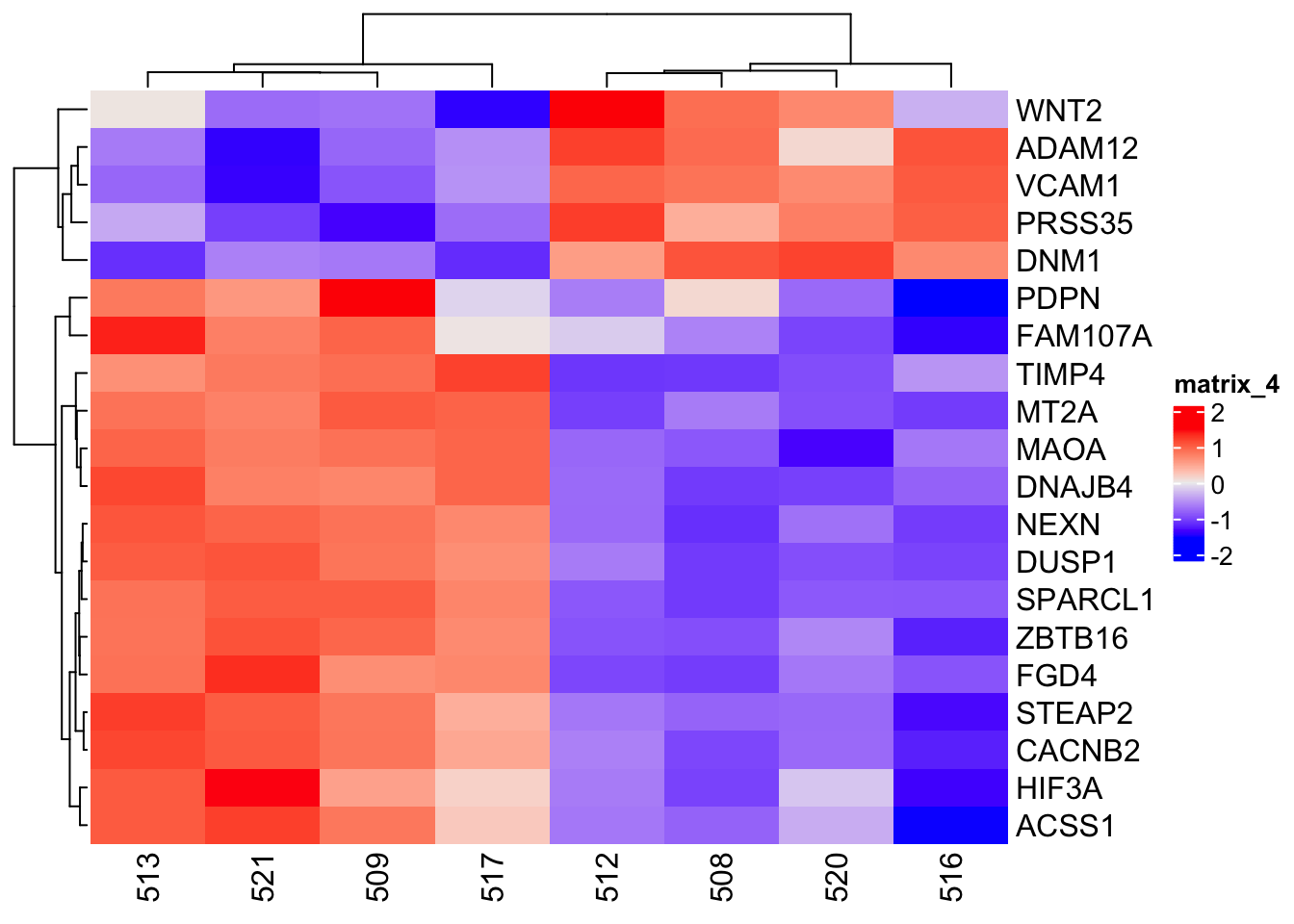
The heatmap for the scaled expression counts data is better at depicting the genes that are differential expressed between the treatment groups.
Heatmap(counts_matrix_scaled)
Step 6: Customizing the heatmap
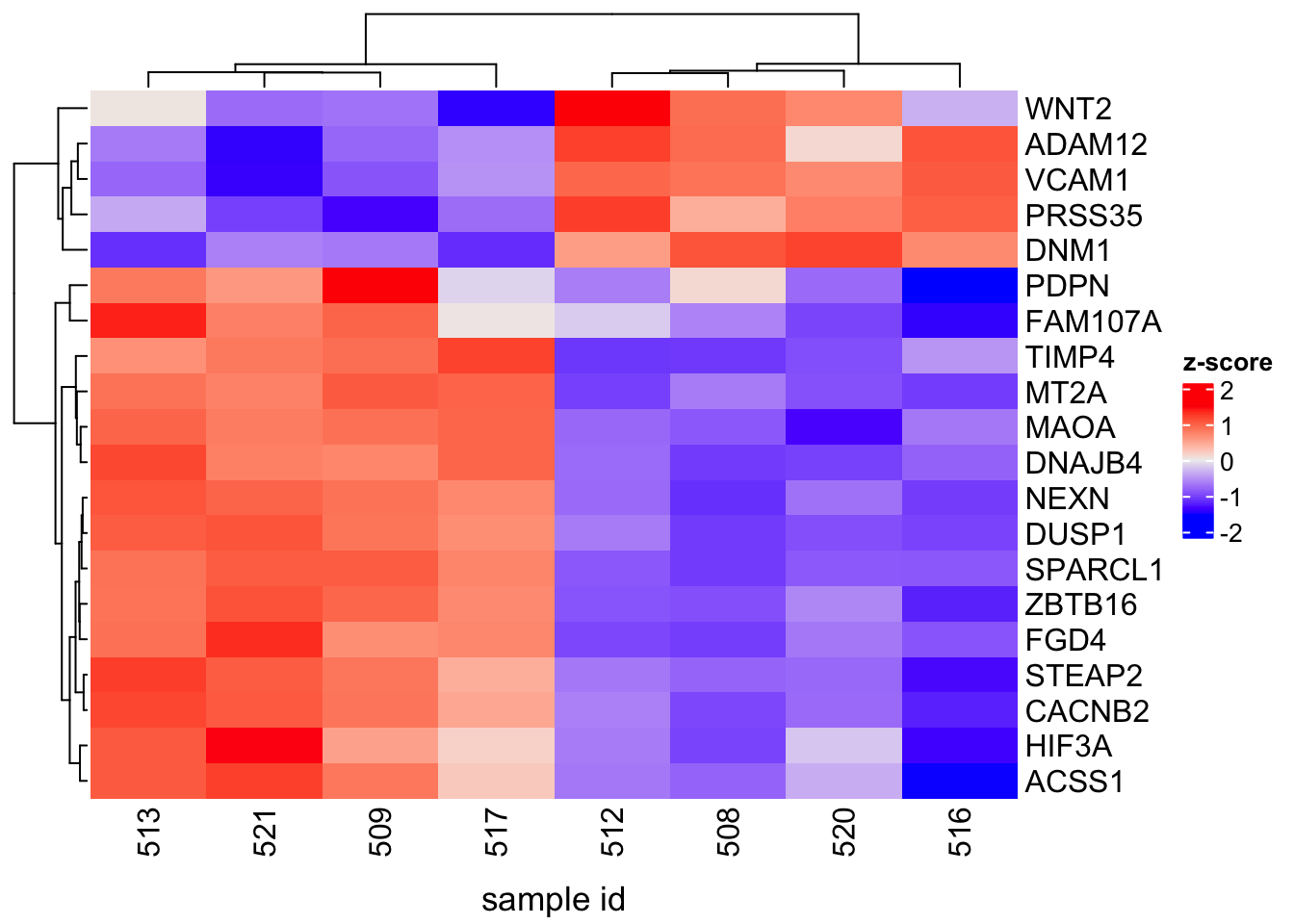
To change the name of the color scale bar, include the name option in the Heatmap command. The name of the color scale bar will be changed to z-score.
Heatmap(counts_matrix_scaled,name="z-score")

To include the title of the columns (ie. title for the bottom horizontal axis), use the column_title option, which will be set to "sample id" so that readers will know that the labels on the bottom horizontal axis of the heatmap refer to sample ids. The column_title_side option tells Heatmap where to place the column title and this will be set to "bottom".
Heatmap(counts_matrix_scaled,name="z-score", column_title="sample id", column_title_side="bottom")
The col option can be used to supply a different coloring scheme. For instance, the Viridis palette is used below.
library(viridis)
Heatmap(counts_matrix_scaled,name="z-score", column_title="samples",
column_title_side="bottom",
col=viridis(10))

## viridis(10) returns 10 colors
It is possible to add an annotation to inform which treatment group the samples came from (ie. control or dexamethasone treated). To do this, create a data frame call samples, where one column lists the sample IDs and the other lists the corresponding treatment group. The tidyverse package will be used for this.
-
The first column in the samples data frame will list the sample identifiers, which can be extracted from the counts_matrix_scaled column headings using
colnames(counts_matrix_scaled), which will then be converted to a data frame usingdata.frame. The commandcolnameswill then be used to set the column heading to "samples" -
ifelsewill then be used to assign the sample identifiers to their treatment groups accordingly.
library(tidyverse)
samples <- data.frame(colnames(counts_matrix_scaled))
colnames(samples) <- "samples"
samples$treatment <- ifelse(samples$samples %in% c("508","512","516","520"), "untreated","treated")
Call the samples data frame to see what it looks like.
samples
  samples treatment
1     508 untreated
2     509   treated
3     512 untreated
4     513   treated
5     516 untreated
6     517   treated
7     520 untreated
8     521   treated
Next, create annotations using the function HeatmapAnnotation from ComplexHeatmap. This annotation will be stored as my_annotations. Inside HeatmapAnnotation, the following is provided:
-
Variable dex, which is set to the treatment column in the data frame samples.
-
The option
col,which assigns color to the different treatment groups.
In the Heatmap command, the option top_annotation is included and this is set to my_annotation.
my_annotations <- HeatmapAnnotation(dex=samples$treatment,
col=list(dex=c("untreated"="blue","treated"="orangered")))

Heatmap(counts_matrix_scaled,name="z-score", column_title="samples",
column_title_side="bottom",
col=viridis(10),
top_annotation=my_annotations)

To fine tune the heatmap, options that allow for changing of font sizes will be included in the annotation (my_annotations) and within the Heatmap command.
In my_annotations, add the following options
annotation_legend_paramis used to set the legend title and text font size. This option takes a list as input and the list contains graphical parameters (title_gpandlabel_gp) that can be used to alter the font size for the annotation legend title and labels.
In the Heatmap command:
-
column_title_gp: a graphical parameter that allows for setting of column title font size. -
column_dend_heightandrow_dend_width: graphical parameters that allow for setting the height and width, respectively for the column and row dendrograms. -
row_names_gpandcolumn_names_gp: graphical parameters that allow for setting of font size for the row and column names, respectively. -
heatmap_legend_param: takes a list that contains options for changing the heatmap legend title font size (title_gp) and legend text font size (label_gp)
my_annotations <- HeatmapAnnotation(dex=samples$treatment,
col=list(dex=c("untreated"="blue","treated"="orangered")),
annotation_legend_param=list(title_gp=gpar(fontsize=16), label_gp=gpar(fontsize=16)))

Heatmap(counts_matrix_scaled,name="z-score", column_title="samples",
column_title_side="bottom",
col=viridis(10),
top_annotation=my_annotations,
column_title_gp=gpar(fontsize=16),
column_dend_height=unit(1,"cm"),
row_dend_width=unit(1.5,"cm"),
row_names_gp=gpar(fontsize=10),
column_names_gp=gpar(fontsize=16),
heatmap_legend_param=list(title_gp=gpar(fontsize=16),
label_gp=gpar(fontsize=16)))
ComplexHeatmap has lots of other capabilities. These include multi-panel heatmaps, OncoPrint, UpSet plots, and more elegant as well as complex genomic heatmaps. Users are encouraged to refer to the ComplexHeatmap user guide to learn more.
Background on volcano plot
A volcano plot is a special case of a scatter plot. It is used in RNA sequencing analysis to visualize gene expression change versus statistical significance of gene expression change.
The differential expression analysis results from the Airway study will be used to explore construction of volcano plots using the EnhancedVolcano package.
Step-by-step guide to making a volcano plot
Step 1: Import the data
my_file <- paste0(data_path,"/","airway_deg_results.csv")
airway_deg <- read.csv(my_file,check.names=FALSE,row.names=1)
EnhancedVolcano is easy to use. All users have to do is to provide it with
-
A data frame containing the differential expression analysis results.
-
The row names of the differential expression analysis results table, which contains the gene identifiers. These will be used to label points on the volcano plot.
-
The column in the differential expression analysis results table that has the expression change values (ie. log2FoldChange).
-
The column in the differential expression analysis results table that has the statistical confidence values for the gene expression change (ie. adjusted P value). Note that the y-axis on the enhanced volcano plot is the negative log10 of the P value. Typically, users will need to calculate and place this in a column in the differential expression results table. However, with EnhancedVolcano, this is done for the user.
EnhancedVolcano also has a default set of gene expression change and statistical confidence cutoffs that determine whether gene expression has no significant change (NS, gray points), meets expression change criteria (Log2 FC, green points), statistical confidence criteria (p-value, blue points), or both expression change and statistical confidence criteria (p-value and log2 FC, pink points). Users would need to include this information in a column of the differential expression results table if constructing the volcano plot using another tool.
Step 2: Load the EnhancedVolcano package
library(EnhancedVolcano)
Step 3: Construct the volcano plot using the command EnhancedVolcano with the following arguments
-
Argument: airway_deg (the data frame containing the differential expression analysis results)
-
Argument:
lab, which is set to the row names of the airway_deg data frame. The row names of the airway_deg data frame contains the gene identifiers. -
Argument:
xaxis value, which is set to log2FoldChange -
Argument:
yaxis value, which is set to padj
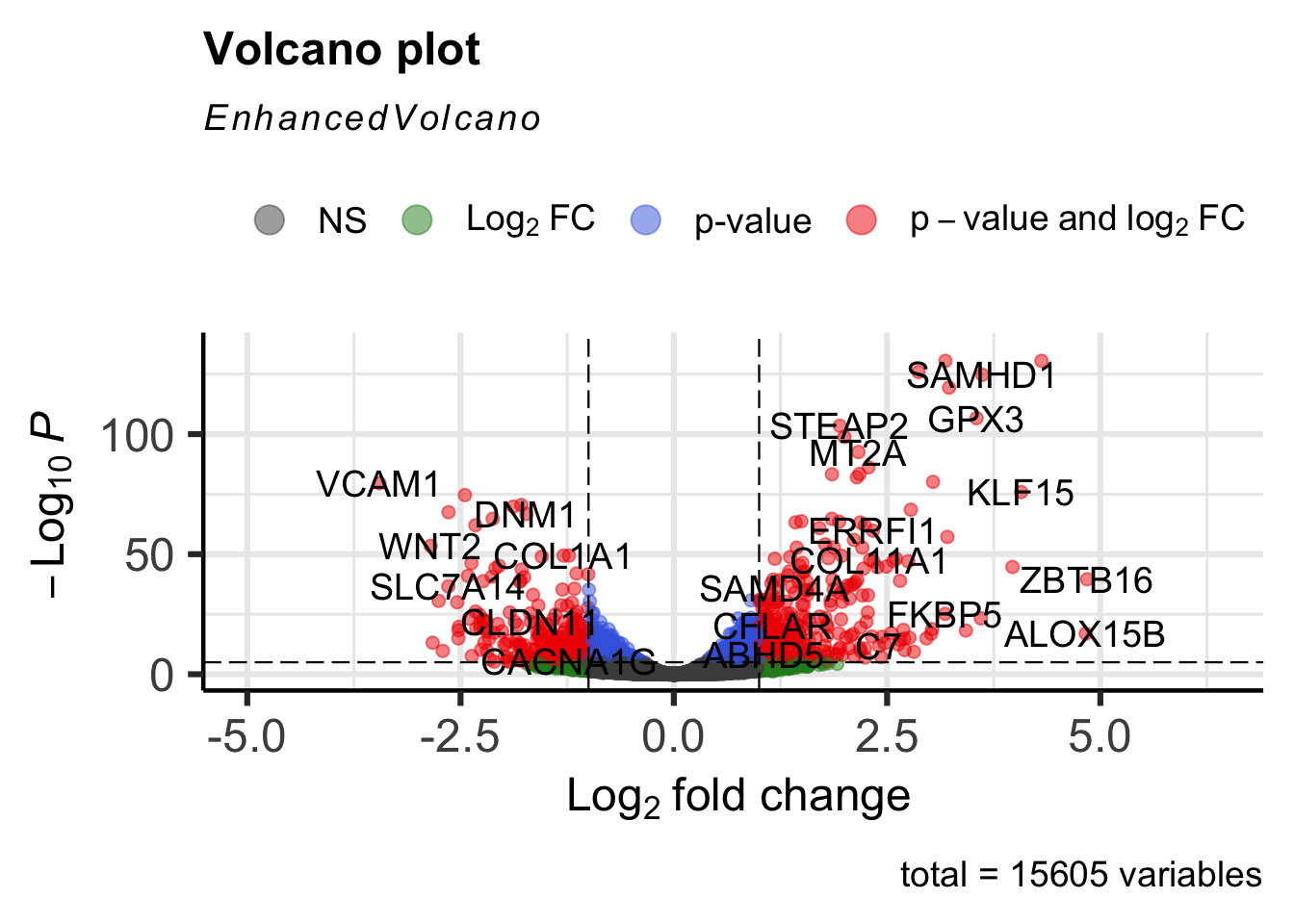
EnhancedVolcano(airway_deg,lab=rownames(airway_deg),x="log2FoldChange",y="padj")
Step 4: Customizing the volcano plot
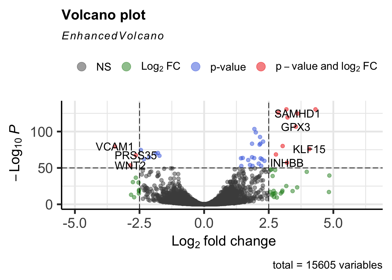
The pCutoff and FCcutoff options can be used to specify the p-value and fold change cutoff criteria for a gene to be classified as significantly up or down regulated.
EnhancedVolcano(airway_deg,lab=rownames(airway_deg),x="log2FoldChange",y="padj",
pCutoff=1e-50, FCcutoff=2.5)
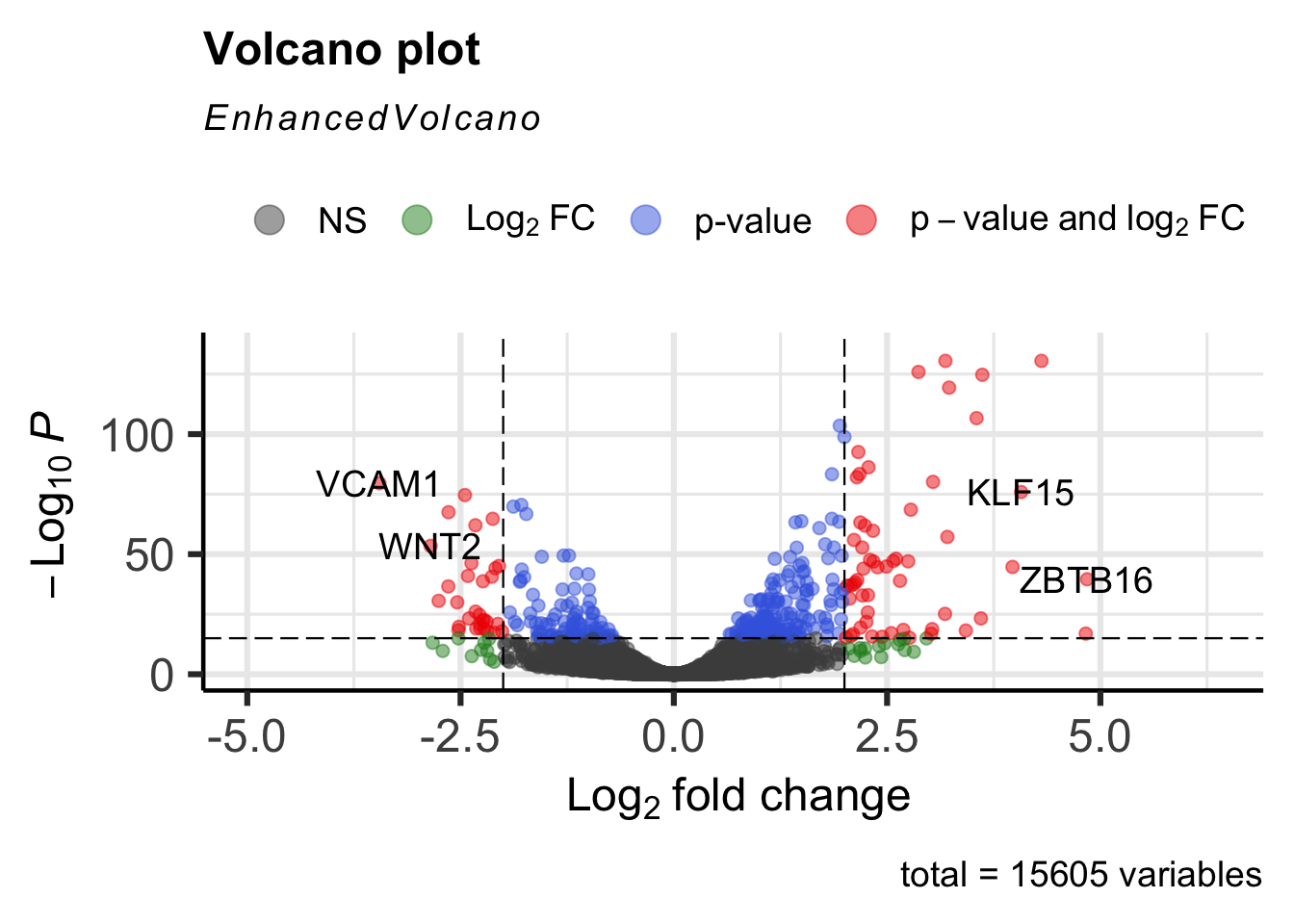
Include the selectLab option to specify a custom list of genes to label.
EnhancedVolcano(airway_deg,lab=rownames(airway_deg),x="log2FoldChange",y="padj",
pCutoff=1e-15, FCcutoff=2,
selectLab=c("VCAM1", "WNT2", "KLF15", "ZBTB16"))
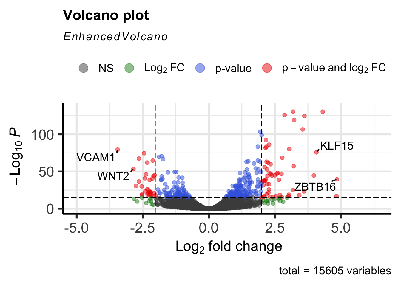
Set drawConnectors to TRUE to add a connecting arrow that points to the gene label. This also positions the gene label so that it does not overlap the point.
EnhancedVolcano(airway_deg,lab=rownames(airway_deg),x="log2FoldChange",y="padj",
pCutoff=1e-15, FCcutoff=2,
selectLab=c("VCAM1", "WNT2", "KLF15", "ZBTB16"),
drawConnectors=TRUE)
Use the title and subtitle options to set a title and subtitle, respectively for the volcano plot. The col option can be included to specify a custom list of legend colors. In the example below, everything is in black except for the genes that exhibit statistically significant expression change by meeting both the p-value and fold change cutoffs.
EnhancedVolcano(airway_deg,lab=rownames(airway_deg),x="log2FoldChange",y="padj",
pCutoff=1e-15, FCcutoff=2,
selectLab=c("VCAM1", "WNT2", "KLF15", "ZBTB16"),
drawConnectors=TRUE,
title="Dexmethasone treated vs untreated",
subtitle="Differential expression",
col=c("black","black","black","red"))

Class dataset
Download a zip folder containing the data used in class to practice
The folder contains:
- RNAseq_mat_top20.csv: log2 CPM expression values for the top 20 differential expressed genes in the Airway study.
- airway_deg_results.csv: differential expression analysis results for the Airway study.