Functional Enrichment Analysis with clusterProfiler
Learning Objectives
- Understand the capabilities of
clusterProfilerin the context of functional enrichment analysis - Learn about related packages to improve results reporting
What is Functional Enrichment Analysis?
Functional enrichment and pathway analysis have broad and varying definitions. For our purposes, there are three general approaches (Khatri et al. 2012):
- Over-Representation Analysis (ORA)
- Functional Class Scoring (FCS)
- Pathway Topology (PT)
Over-representation analysis (ORA)
statistically evaluates the fraction of genes in a particular pathway found among the set of genes showing changes in expression --- Khatri et al. 2012
From this, ORA determines which pathways are over or under represented by asking "are there more annotations in the gene list than expected?"
- tests based on hypergeometric, chi-square, or binomial distribution
- includes GO enrichment methods
- prioritizes a subset of genes using an arbitrary, user determined threshold (e.g., p-value)
- doesn't require the data, just the gene identifiers
- not great for gene lists with less than 50 genes
Functional Class Scoring (FCS)
Includes ‘gene set scoring’ methods such as GSEA, which first compute DE scores for all genes measured, and subsequently compute gene set scores by aggregating the scores of contained genes. --- Geistlinger et al. 2021
GSEA
- ignore gene position and role
- do not pre-select genes (considers all gene expression) and so you must include data with gene identifiers for ranking
- ranking by magnitude of change in gene expression between conditions
- determines where genes from a gene set fall in the ranking
- creates a running sum statistic
- uses a permutational approach to determine significance
- Broad Institute software but also available using web-based tools, R, and Qlucore (proprietary).
- also considered a strategy encompassing a range of methods
- self-contained methods vs competitive methods
Pathway Topology
ORA and FCS discard a large amount of information. These methods use gene sets, and even if the gene sets represent specific pathways, structural information such as gene product interactions, positions of genes, and types of genes is completely ignored. Pathway topology methods seek to rectify this problem.
PT methods are mostly considered network based.
Some examples:
Impact analysis (iPathwayGuide), Pathway-Express, SPIA, NetGSA, etc. (See Nguyen et al. 2019 for a review of PT methods.)
What is clusterProfiler?
clusterProfiler is an R package used for functional enrichment analysis (either ORA or GSEA). See the latest publication here. The primary documentation for clusterProfiler can be found here.
Advantages of clusterProfiler
- ORA and GSEA support
- Functionality for multiple ontology and pathway databases
- Allows user defined databases and annotations, which is particularly useful for non-model organisms
- Easily compare functional profiles between treatments
- integrates the tidy philosophy
- complementary packages (
ChIPseeker,GOSemSim,enrichplot,ReactomePA,DOSE) provide a comprehensive tool suite for understanding functional enrichment.

Load dependencies
library(clusterProfiler)
library(org.Hs.eg.db)
library(tidyverse)
library(DOSE)
library(ReactomePA)
library(enrichplot)
The Dataset
For today's lesson, we will use data derived from the Bioconductor package airway. The airway data is from Himes et al. (2014). These data, which are contained within a RangedSummarizedExperiment, object are from a bulk RNAseq experiment. In the experiment, the authors "characterized transcriptomic changes in four primary human ASM cell lines that were treated with dexamethasone," a common therapy for asthma. The airway package includes RNAseq count data from 8 airway smooth muscle cell samples. Each cell line includes a treated and untreated negative control. Differential expression testing using DESeq2 was applied to these data. You can download the differential expression results here.
Load the differential expression results:
dexp<-read.csv("../data/S3_clusterProfiler/deseq2_DEGs.csv")
colnames(dexp)[1]<-"Ensembl"
Create gene lists:
# Extract all significant results for ORA
sigDEGs <- dplyr::filter(dexp, padj < 0.05)
# limiting results by log2FoldChange; may want to use log2FoldChange<0
sig_down<- dplyr::filter(dexp, padj < 0.05 & log2FoldChange < -1)
# limiting results by log2FoldChange; may want to use log2FoldChange>0
sig_up<- dplyr::filter(dexp, padj < 0.05 & log2FoldChange > 1)

# Rank results for GSEA; put in decreasing order.
GSEA_data<-dexp %>% filter(!is.na(padj)) %>%
  arrange(desc(log2FoldChange)) %>%
  # create a named vector with log fold changes
  pull(log2FoldChange,name=symbol)
Annotations
We have already mapped gene symbols and Entrez IDs to our data using AnnotationDbi and EnsDb.Hsapiens.v75. However, clusterProfiler does offer support for gene ID conversion using the functions bitr() and bitr_kegg(). bitr() uses the OrgDb packages, of which there are 19 databases. bitr_kegg() unsurprisingly uses KEGG organism annotations. Use search_kegg_organism() to find the appropriate kegg code.
For example:
#get keytype info
keytypes(org.Hs.eg.db)
 [1] "ACCNUM"       "ALIAS"        "ENSEMBL"      "ENSEMBLPROT"  "ENSEMBLTRANS"
 [6] "ENTREZID"     "ENZYME"       "EVIDENCE"     "EVIDENCEALL"  "GENENAME"
[11] "GENETYPE"     "GO"           "GOALL"        "IPI"          "MAP"
[16] "OMIM"         "ONTOLOGY"     "ONTOLOGYALL"  "PATH"         "PFAM"
[21] "PMID"         "PROSITE"      "REFSEQ"       "SYMBOL"       "UCSCKG"
[26] "UNIPROT"
#need entrez IDs?
ids<-bitr(sigDEGs$Ensembl, fromType="ENSEMBL",
          toType="ENTREZID",
          OrgDb="org.Hs.eg.db") #NA values drop by default
'select()' returned 1:many mapping between keys and columns
Warning in bitr(sigDEGs$Ensembl, fromType = "ENSEMBL", toType = "ENTREZID", :
5.31% of input gene IDs are fail to map...
#view
head(ids)
          ENSEMBL ENTREZID
1 ENSG00000152583     8404
2 ENSG00000165995      783
3 ENSG00000120129     1843
4 ENSG00000101347    25939
5 ENSG00000189221     4128
6 ENSG00000211445     2878
Note
clusterProfiler functions are fully supported by OrgDb and you can provide a Keytype argument within functions.
Over-representation analysis with clusterProfiler
clusterProfiler, along with complementary packages, can easily be used to generate functional enrichment results using over-representation analysis from the following databases: GO, KEGG, DOSE, REACTOME, Wikipathways, DisGeNET, network of cancer genes.
Using ?enrichGO()
GO enrichment refers specifically to gene ontology.
The Gene Ontology (GO) provides a framework and set of concepts for describing the functions of gene products from all organisms. --- https://www.ebi.ac.uk/ols/ontologies/go.
GO integrates information about gene product function in the context of three domains:
- molecular function (F) - "the molecular activities of individual gene products" (e.g., kinase)
- cellular component (C) - "where the gene products are active" (e.g., mitochondria)
- *biological process (P) - "the pathways and larger processes to which that gene product’s activity contributes" (e.g., transport)
*Commonly used for pathway enrichment analysis
GO terms can be highly redundant, and GO enrichment analysis often requires us to deal with this redundancy (See below).
Checkout geneontology.org.
Read more about GO enrichment analysis with clusterProfiler here.
Let's perform GO enrichment on our up-regulated genes. Notice that OrgDB databases and keyType can be specified directly in the function. In addition, you can specify a list of background genes or use the default which will use all genes in the queried database (e.g., GO-BP). Here we are specifying the genes that underwent differential expression testing, but there is currently an open issue on the way the universe is affecting results, which can impact significance values.
ego <- enrichGO(gene= sig_up$symbol,
                OrgDb= org.Hs.eg.db,
                keyType = "SYMBOL",
                ont= "BP",
                universe=dexp$symbol)
Note
If we want to included all three ontologies (i.e., MF, CC, and BP), we can do so with ont= "ALL".
Let's take a peek at the results:
ego
#
# over-representation test
#
#...@organism    Homo sapiens
#...@ontology    BP
#...@keytype     SYMBOL
#...@gene    chr [1:451] "SPARCL1" "CACNB2" "DUSP1" "SAMHD1" "MAOA" "GPX3" "STEAP2" ...
#...pvalues adjusted by 'BH' with cutoff <0.05
#...53 enriched terms found
'data.frame':   53 obs. of  9 variables:
 $ ID         : chr  "GO:0003012" "GO:0045444" "GO:0030198" "GO:0043062" ...
 $ Description: chr  "muscle system process" "fat cell differentiation" "extracellular matrix organization" "extracellular structure organization" ...
 $ GeneRatio  : chr  "27/351" "18/351" "21/351" "21/351" ...
 $ BgRatio    : chr  "374/14114" "207/14114" "277/14114" "278/14114" ...
 $ pvalue     : num  7.27e-07 4.25e-06 6.02e-06 6.37e-06 6.73e-06 ...
 $ p.adjust   : num  0.00266 0.00493 0.00493 0.00493 0.00493 ...
 $ qvalue     : num  0.00238 0.0044 0.0044 0.0044 0.0044 ...
 $ geneID     : chr  "CACNB2/KLF15/ERRFI1/FOXO1/PDLIM5/LMCD1/LMOD1/NR4A3/SCN7A/ABCC9/OXTR/APBB2/ABAT/FOXO3/CFLAR/ACTA2/LEP/ATP2A2/GDN"| __truncated__ "SORT1/INHBB/ZBTB16/FOXO1/CEBPD/NR4A3/STEAP4/KLF5/LEP/CCDC71L/ALDH6A1/AXIN2/FRZB/NR4A1/LMO3/DIO2/FABP4/ENPP1" "ADAMTS1/PDPN/PTX3/LAMA2/COL11A1/CRISPLD2/GPM6B/COL4A1/COL4A4/CFLAR/NID1/ITGA8/DPT/SPINT2/ANGPTL7/MMP15/COL4A3/A"| __truncated__ "ADAMTS1/PDPN/PTX3/LAMA2/COL11A1/CRISPLD2/GPM6B/COL4A1/COL4A4/CFLAR/NID1/ITGA8/DPT/SPINT2/ANGPTL7/MMP15/COL4A3/A"| __truncated__ ...
 $ Count      : int  27 18 21 21 21 8 23 27 8 10 ...
#...Citation
 T Wu, E Hu, S Xu, M Chen, P Guo, Z Dai, T Feng, L Zhou, W Tang, L Zhan, X Fu, S Liu, X Bo, and G Yu.
 clusterProfiler 4.0: A universal enrichment tool for interpreting omics data.
 The Innovation. 2021, 2(3):100141
We have 53 significantly enriched terms (p.adjust < 0.05, log2foldchange > 1) that are up-regulated in response to dexamethasone treatment.
What do we need to know about the output from enrichGO()?
Some of the columns are self-explanatory, while others are not:
GeneRatio (k/n): "ratio of input genes that are annotated in a term." (# of genes in the input list that are annotated to the corresponding term (function) / # of genes in input list).
BgRatio (M/N): "ratio of all genes that are annotated in this term" (The number of genes that are annotated to the term / The total number of genes in the background gene list ("universe")).
pvalue: over-representation assessed using hypogeometric distribution, which is equivalent to a one sided Fisher's exact test.
p.adjust: Hypergeometric p-value after correction for multiple testing ("BH adjusted p-values"); see ?p.adjust.
qvalue: another take on FDR adjusted p-values; See ?qvalue::qvalue.
geneID: The gene IDs that overlap with the functional term.
Count: Total number of genes from the input gene list that match the functional term.
Info
p.adjust may potentially be more conservative and robust than q-value. See the following discussions:
- conceptual question about FDR, FDR adjusted p-value and q-value
- Why use the qvalue package instead of p.adjust in R stats?
Reduce redundancy
Because of the nature of GO, organized as a directed acyclic graph, parent terms can show enrichment due to over represented child terms. To reduce redundancy among enriched terms, clusterProfiler uses a simplify() function that uses the "GOSemSim package to calculate semantic similarities among enriched GO terms using multiple methods based on information content or graph structure." GO terms with >0.7 similarity are removed and represented by the most significant term (Wu et al. 2021).
Let's reduce our GO terms using simplify().
s_ego<-clusterProfiler::simplify(ego)
s_ego
#
# over-representation test
#
#...@organism    Homo sapiens
#...@ontology    BP
#...@keytype     SYMBOL
#...@gene    chr [1:451] "SPARCL1" "CACNB2" "DUSP1" "SAMHD1" "MAOA" "GPX3" "STEAP2" ...
#...pvalues adjusted by 'BH' with cutoff <0.05
#...35 enriched terms found
'data.frame':   35 obs. of  9 variables:
 $ ID         : chr  "GO:0003012" "GO:0045444" "GO:0030198" "GO:0043062" ...
 $ Description: chr  "muscle system process" "fat cell differentiation" "extracellular matrix organization" "extracellular structure organization" ...
 $ GeneRatio  : chr  "27/351" "18/351" "21/351" "21/351" ...
 $ BgRatio    : chr  "374/14114" "207/14114" "277/14114" "278/14114" ...
 $ pvalue     : num  7.27e-07 4.25e-06 6.02e-06 6.37e-06 6.73e-06 ...
 $ p.adjust   : num  0.00266 0.00493 0.00493 0.00493 0.00493 ...
 $ qvalue     : num  0.00238 0.0044 0.0044 0.0044 0.0044 ...
 $ geneID     : chr  "CACNB2/KLF15/ERRFI1/FOXO1/PDLIM5/LMCD1/LMOD1/NR4A3/SCN7A/ABCC9/OXTR/APBB2/ABAT/FOXO3/CFLAR/ACTA2/LEP/ATP2A2/GDN"| __truncated__ "SORT1/INHBB/ZBTB16/FOXO1/CEBPD/NR4A3/STEAP4/KLF5/LEP/CCDC71L/ALDH6A1/AXIN2/FRZB/NR4A1/LMO3/DIO2/FABP4/ENPP1" "ADAMTS1/PDPN/PTX3/LAMA2/COL11A1/CRISPLD2/GPM6B/COL4A1/COL4A4/CFLAR/NID1/ITGA8/DPT/SPINT2/ANGPTL7/MMP15/COL4A3/A"| __truncated__ "ADAMTS1/PDPN/PTX3/LAMA2/COL11A1/CRISPLD2/GPM6B/COL4A1/COL4A4/CFLAR/NID1/ITGA8/DPT/SPINT2/ANGPTL7/MMP15/COL4A3/A"| __truncated__ ...
 $ Count      : int  27 18 21 21 21 8 23 27 10 8 ...
#...Citation
 T Wu, E Hu, S Xu, M Chen, P Guo, Z Dai, T Feng, L Zhou, W Tang, L Zhan, X Fu, S Liu, X Bo, and G Yu.
 clusterProfiler 4.0: A universal enrichment tool for interpreting omics data.
 The Innovation. 2021, 2(3):100141
We are now left with 35 enriched terms.
Visualize results using enrichplot a complementary package of clusterProfiler
enrichplot is based on ggplot2 implementation. Therefore, all plots can be customized with ggplot2 functions.
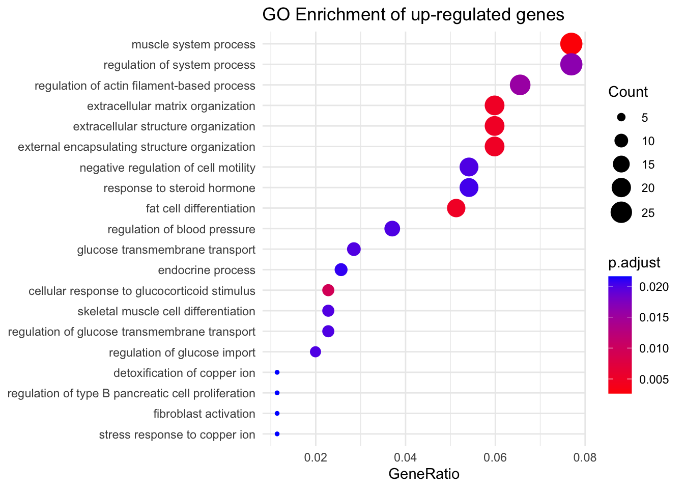
Dotplot
Plot results using a dotplot.
dotplot(s_ego,showCategory=20,font.size=10,label_format=70)+
  scale_size_continuous(range=c(1, 7))+
  theme_minimal() +
  ggtitle("GO Enrichment of up-regulated genes")
Scale for size is already present.
Adding another scale for size, which will replace the existing scale.
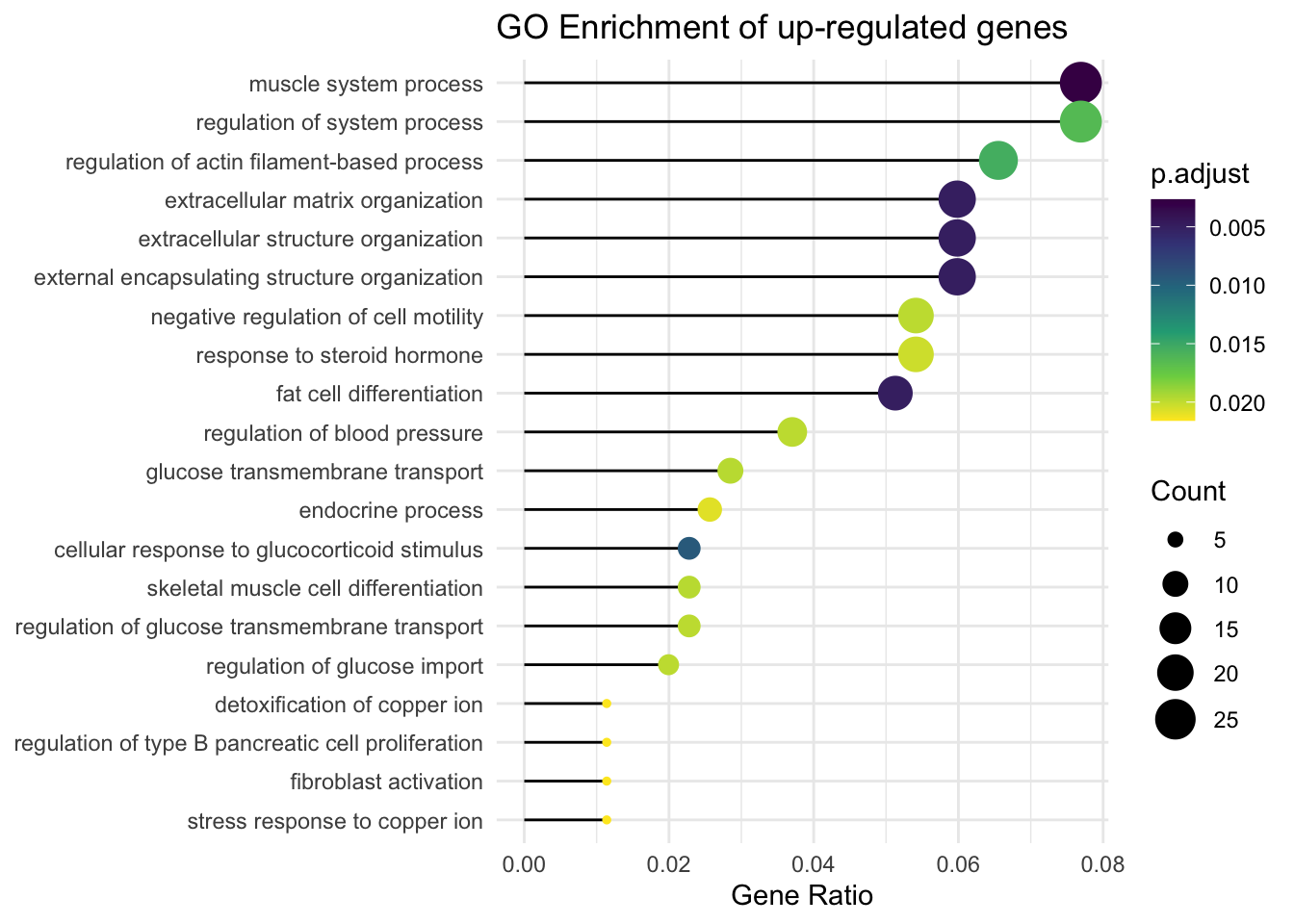
Lollipop plot
These are the same results exhibited differently. Notice the seamless integration with tidyverse functionality. clusterProfiler extends ggplot2 functionality to accept enrichment results directly.
s_ego %>% filter(p.adjust < 0.03) %>%
ggplot(showCategory = 20,
  aes(GeneRatio, forcats::fct_reorder(Description, GeneRatio))) +
  geom_segment(aes(xend=0, yend = Description)) +
  geom_point(aes(color=p.adjust, size = Count)) +
  scale_color_viridis_c(guide=guide_colorbar(reverse=TRUE)) +
  scale_size_continuous(range=c(1, 7)) +
  theme_minimal() +
  xlab("Gene Ratio") +
  ylab(NULL) +
  ggtitle("GO Enrichment of up-regulated genes")
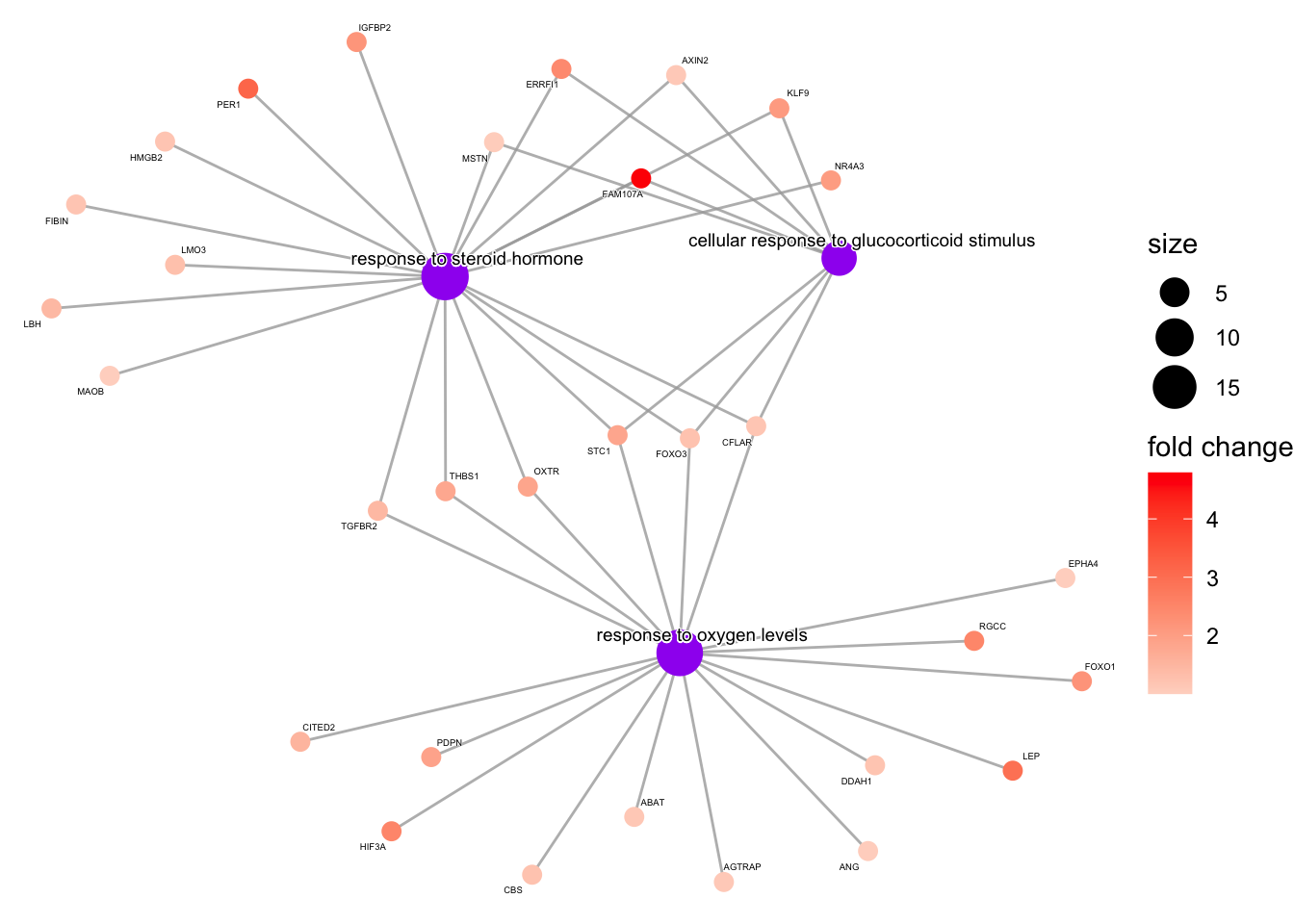
cnetplot
The category netplot (cnetplot) allows us to visualize the relationship and overlap of genes associated with our top terms (or terms that we specify). This is a nice way of visualizing genes that are important for several enriched terms.
# color genes by log2 fold changes; create named vector
foldchanges <- sig_up$log2FoldChange
names(foldchanges) <- sig_up$symbol

## by default cnetplot gives the top 5 significant terms
#if we want to focus on specific terms we can subset our results
s_ego2 <- s_ego
s_ego2@result<-s_ego[c(6,15,32),]

cnetplot(s_ego2,
         foldChange=foldchanges,
         shadowtext='gene',
         cex_label_gene=0.25,
         cex_label_category=0.5,
         color_category="purple")
Warning in cnetplot.enrichResult(x, ...): Use 'color.params = list(foldChange = your_value)' instead of 'foldChange'.
 The foldChange parameter will be removed in the next version.
Warning in cnetplot.enrichResult(x, ...): Use 'color.params = list(category = your_value)' instead of 'color_category'.
 The color_category parameter will be removed in the next version.
Warning in cnetplot.enrichResult(x, ...): Use 'cex.params = list(category_label = your_value)' instead of 'cex_label_category'.
 The cex_label_category parameter will be removed in the next version.
Warning in cnetplot.enrichResult(x, ...): Use 'cex.params = list(gene_label = your_value)' instead of 'cex_label_gene'.
 The cex_label_gene parameter will be removed in the next version.
Scale for size is already present.
Adding another scale for size, which will replace the existing scale.
Note
See how the enrichResult was subset above. These are S4 objects that can be subset using $ and []. To get a quick understanding of the enriched results, we can also use nrow, ncol, and dim.
Other plots with enrichplot
Other plot types possible with enrichplot include barplots, heatmaps (as alternatives to cnetplots), tree plots, enrichment maps, upset plots (alternative to venn diagram), ridgeline plots, and GSEA plots.
Over representation analysis using other databases
Using clusterProfiler you can conduct ORA with GO, KEGG, MKEGG (KEGG modules), and WikiPathways. Using complementary packages (i.e., DOSE, ReactomePA), ORA can also be conducted with Disease Ontology (DO), Reactome, network of cancer genes, and DisGeNET.
#Example with KEGG pathways
kgo <- enrichKEGG(gene = sig_up$entrez,
organism = 'hsa',
pvalueCutoff  = 0.05,
universe = as.character(dexp$entrez)
)
Reading KEGG annotation online: "https://rest.kegg.jp/link/hsa/pathway"...
Reading KEGG annotation online: "https://rest.kegg.jp/list/pathway/hsa"...
kgo_df<-data.frame(kgo)
Note
clusterProfiler uses the latest version of the KEGG database and supports species with KEGG annotation ( > 6000).
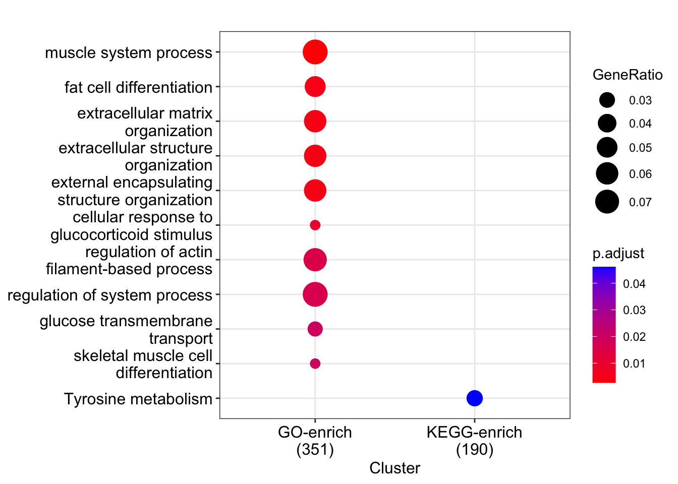
Merge enrichResult
It is possible to merge multiple enrichResult objects; this could be up-regulated merged with down-regulated or different functional repositories.
mlist<-list(s_ego,kgo)
names(mlist)<-c("GO-enrich","KEGG-enrich")
mresult<-merge_result(mlist)
dotplot(mresult,showCategory=10)
Custom ORA using enricher()
There are many databases devoted to relating genes and gene products to pathways, processes, and other phenomenon and a multitude of organisms that may not have annotations in widely used databases (e.g., KEGG, GO). clusterProfiler has generalizable functions that allow users to customize the knowledge database and annotations used for functional enrichment.
Because the gene matrix transposed (GMT) format is often used to share gene set annotations, clusterProfiler provides the parser functions read.gmt() and read.gmt.wp(), the latter of which is specific to Wikipathways.
For example, let's download and use the Molecular Signatures Database (MSigDB) for ORA. In this case, we are interested in the canonical pathways from C2.
C2_cp<-read.gmt("../data/S3_clusterProfiler/c2.cp.v2023.1.Hs.symbols.gmt")
Note
We could also use the package msigdbr to obtain MSigDB gene sets in a tidy format without downloading directly from MSigDB.
Use enricher
Ex <- enricher(sig_up$symbol,
               TERM2GENE = C2_cp,
               universe=dexp$symbol)
head(Ex)
                                                         ID
NABA_CORE_MATRISOME                     NABA_CORE_MATRISOME
PID_INTEGRIN1_PATHWAY                 PID_INTEGRIN1_PATHWAY
WP_COPPER_HOMEOSTASIS                 WP_COPPER_HOMEOSTASIS
BIOCARTA_NPP1_PATHWAY                 BIOCARTA_NPP1_PATHWAY
WP_GABA_METABOLISM_AKA_GHB       WP_GABA_METABOLISM_AKA_GHB
REACTOME_LAMININ_INTERACTIONS REACTOME_LAMININ_INTERACTIONS
                                                Description GeneRatio   BgRatio
NABA_CORE_MATRISOME                     NABA_CORE_MATRISOME    23/296 235/10641
PID_INTEGRIN1_PATHWAY                 PID_INTEGRIN1_PATHWAY    10/296  61/10641
WP_COPPER_HOMEOSTASIS                 WP_COPPER_HOMEOSTASIS     8/296  51/10641
BIOCARTA_NPP1_PATHWAY                 BIOCARTA_NPP1_PATHWAY     4/296  10/10641
WP_GABA_METABOLISM_AKA_GHB       WP_GABA_METABOLISM_AKA_GHB     4/296  10/10641
REACTOME_LAMININ_INTERACTIONS REACTOME_LAMININ_INTERACTIONS     6/296  30/10641
                                    pvalue     p.adjust      qvalue
NABA_CORE_MATRISOME           1.516106e-07 0.0001952744 0.000179858
PID_INTEGRIN1_PATHWAY         6.120069e-06 0.0039413246 0.003630167
WP_COPPER_HOMEOSTASIS         7.335030e-05 0.0269492209 0.024821651
BIOCARTA_NPP1_PATHWAY         1.079261e-04 0.0269492209 0.024821651
WP_GABA_METABOLISM_AKA_GHB    1.079261e-04 0.0269492209 0.024821651
REACTOME_LAMININ_INTERACTIONS 1.488267e-04 0.0269492209 0.024821651
                                                                                                                                                                       geneID
NABA_CORE_MATRISOME           SPARCL1/LAMA2/COL11A1/CRISPLD2/SPON1/IGFBP2/COL7A1/FBN2/MFGE8/COL4A1/OMD/COL4A4/RSPO1/NID1/CILP/CRIM1/DPT/THBS1/LGI3/COL4A3/HAPLN3/PRG4/COL28A1
PID_INTEGRIN1_PATHWAY                                                                                       LAMA2/COL11A1/COL7A1/COL4A1/COL4A4/NID1/ITGA10/ITGA8/THBS1/COL4A3
WP_COPPER_HOMEOSTASIS                                                                                                         STEAP2/MT2A/STEAP1/FOXO1/MT1E/STEAP4/FOXO3/MT1X
BIOCARTA_NPP1_PATHWAY                                                                                                                              COL4A1/COL4A4/COL4A3/ENPP1
WP_GABA_METABOLISM_AKA_GHB                                                                                                                               ABAT/GLS/ADHFE1/MAOB
REACTOME_LAMININ_INTERACTIONS                                                                                                          LAMA2/COL7A1/COL4A1/COL4A4/NID1/COL4A3
                              Count
NABA_CORE_MATRISOME              23
PID_INTEGRIN1_PATHWAY            10
WP_COPPER_HOMEOSTASIS             8
BIOCARTA_NPP1_PATHWAY             4
WP_GABA_METABOLISM_AKA_GHB        4
REACTOME_LAMININ_INTERACTIONS     6
This requires a TERM2GENE argument. This argument accepts a data frame with two columns: "term" and "gene". "term" includes the term ID, while "gene" includes the mapped gene associated with that term. You may also want to include a TERM2NAME argument, which is a dataframe with a column for the term ID and the term name.
GSEA
The complementary function for a customized GSEA, rather than ORA, is GSEA().
Gene set files
Enrichr has a fantastic library of potential gene sets of interest.
Compare functional profiles between conditions
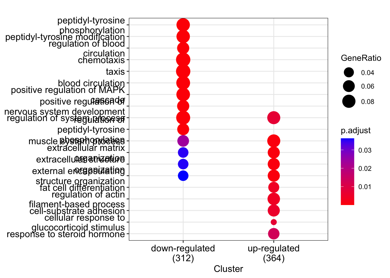
clusterProfiler is great at biological theme comparison. The function, compareCluster, allows us to compare multiple conditions, time points, experiments, etc. "Comparing functional profiles can reveal functional consensus and differences among different experiments and helps in identifying differential functional modules in omics datasets" (Wu et al. 2021)
This function takes a list of gene lists from the different conditions we want to compare, creates functional enrichment profiles for each list, and combines the results in a single file that can easily be visualized. Alternatively, you can provide a formula (see here).
comparelist<-list(sig_down$Ensembl,sig_up$Ensembl)
names(comparelist)<-c("down-regulated","up-regulated")
cclust<-compareCluster(geneCluster = comparelist,
               fun = enrichGO,
               OrgDb= org.Hs.eg.db,
               keyType = "ENSEMBL",
               ont= "BP",
               universe=dexp$Ensembl)
Visualize results with a dotplot.
dotplot(cclust,showCategory=10)
GSEA with clusterProfiler
clusterProfiler also supports the Broad Institute software method of gene set enrichment analysis (GSEA) developed by Subramanian et al. 2005. Because this method uses all of the data (complete ranked gene list), this method is able to unveil situations where genes within a gene set "change in a small but coordinated way" (i.e., all of the data is used regardless of arbitrary cut-offs like p-values).
GSEA requires an ordered ranked gene list as input.
View GSEA_data
head(GSEA_data)
      ALOX15B        ZBTB16        GUCY2D RP11-357D18.1        STEAP4
    10.970146      7.273192      6.449094      6.184841      5.112808
      ANGPTL7
     4.823511
Method outputs
-
Enrichment Score and normalized enrichment score.
Enrichment Score - represents the degree to which a set is over-represented at the top or bottom of the ranked list.
normalized enrichment score (NES) - allows comparability across gene sets by accounting for differences in gene set size and in correlations between gene sets and the expression dataset. A positive NES is associated with pathway activation, and a negative NES is associated with pathway suppression.
-
Significance calculation (pvalue) using a permutation test on gene labels.
- Adjustment of multiple hypothesis testing (p.adjust) and FDR control (qvalue).
Leading edge analysis outputs:
The leading edge subset of a gene set is the subset of members that contribute most to the ES. For a positive ES, the leading edge subset is the set of members that appear in the ranked list prior to the peak score. For a negative ES, it is the set of members that appear subsequent to the peak score. --- GSEAUserGuide
Leading_edge:
tags - the percentage of genes before or after the peak in the running enrichment score, which is an indication of the percentage of genes contributing to the enrichment score.
list - where in the list the enrichment score is attained.
signal - enrichment signal strength.
core_enrichment:
Returns the core enriched genes, those that contribute the most to a given gene set.
Note
The gene label permutation step uses random reordering. Results may differ between runs if you do not use a random seed generator (e.g., set.seed()).
Similar to ORA, GSEA can be performed using GO (gseGO), KEGG pathways (gseKEGG), KEGG modules (gseMKEGG), and WikiPathways (gseWP). With the DOSE package, you can also use gseDGN, gseDO, and gseNCG, and with ReactomePA (gsePathway).
There is also a customizable function similar to enricher, which is GSEA().
GSEA using GO (gseGO())
set.seed(123)
gsea_go <- gseGO(geneList = GSEA_data,
              OrgDb = org.Hs.eg.db,
              ont = "BP",
              keyType = "SYMBOL",
              seed=TRUE)
preparing geneSet collections...
GSEA analysis...
Warning in preparePathwaysAndStats(pathways, stats, minSize, maxSize, gseaParam, : There are ties in the preranked stats (0.05% of the list).
The order of those tied genes will be arbitrary, which may produce unexpected results.
leading edge analysis...
done...
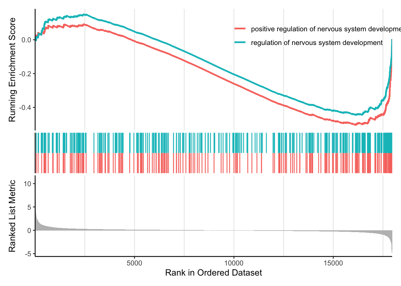
Plot GSEA results
enrichplot offers several functions specific to GSEA output, especially in regard to visualizing the running score and preranked list (gseaplot() and gseaplot2()). gseaplot2() allows us to visualize several enriched gene sets at once.
enrichplot::gseaplot2(gsea_go, geneSetID = c(1:2))
enrichplot::gseaplot2(gsea_go, geneSetID = c(29,35))

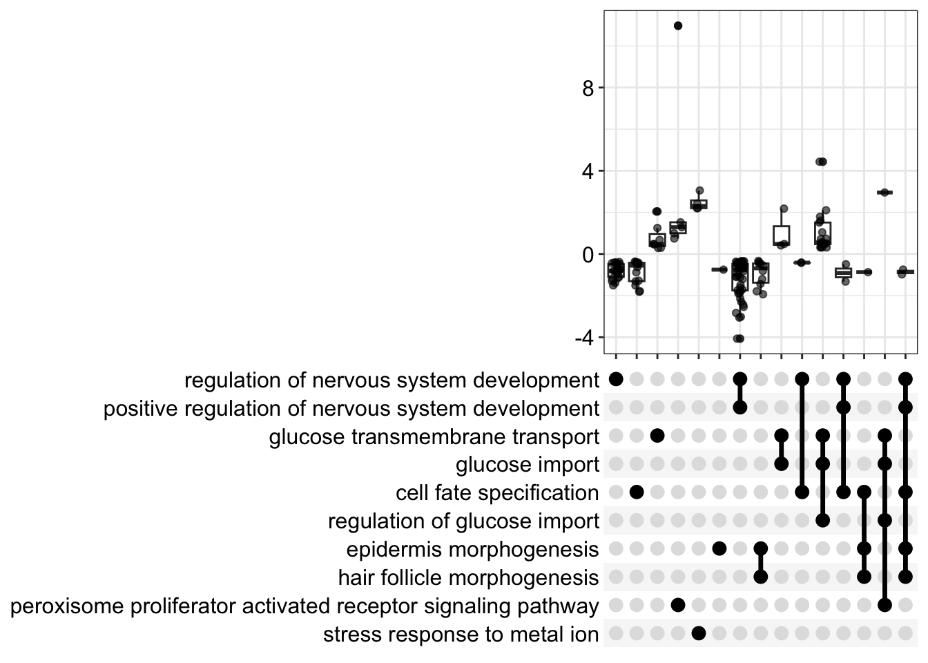
We can use an upset plot to look at fold distributions over gene sets. This requries the installation of the ggupset package.
enrichplot::upsetplot(gsea_go)
Note
Other enrichplot functions can also be applied to GSEA outputs (e.g., dotplot, cnetplot, enrichmap, etc.) or we can use the ggplot2 functionality.
Using clusterProfiler dplyr verb extensions
We can use clusterProfiler extensions of dplyr verbs (mutate(),filter(),select(),summarize(),slice(),group_by(),arrange()) for easy manipulation of enrichResult, gseaResult, and compareClusterResult objects. mutate() can be particularly powerful and allow us to use different enrichment result metrics (e.g., rich factor and fold enrichment for ORA).
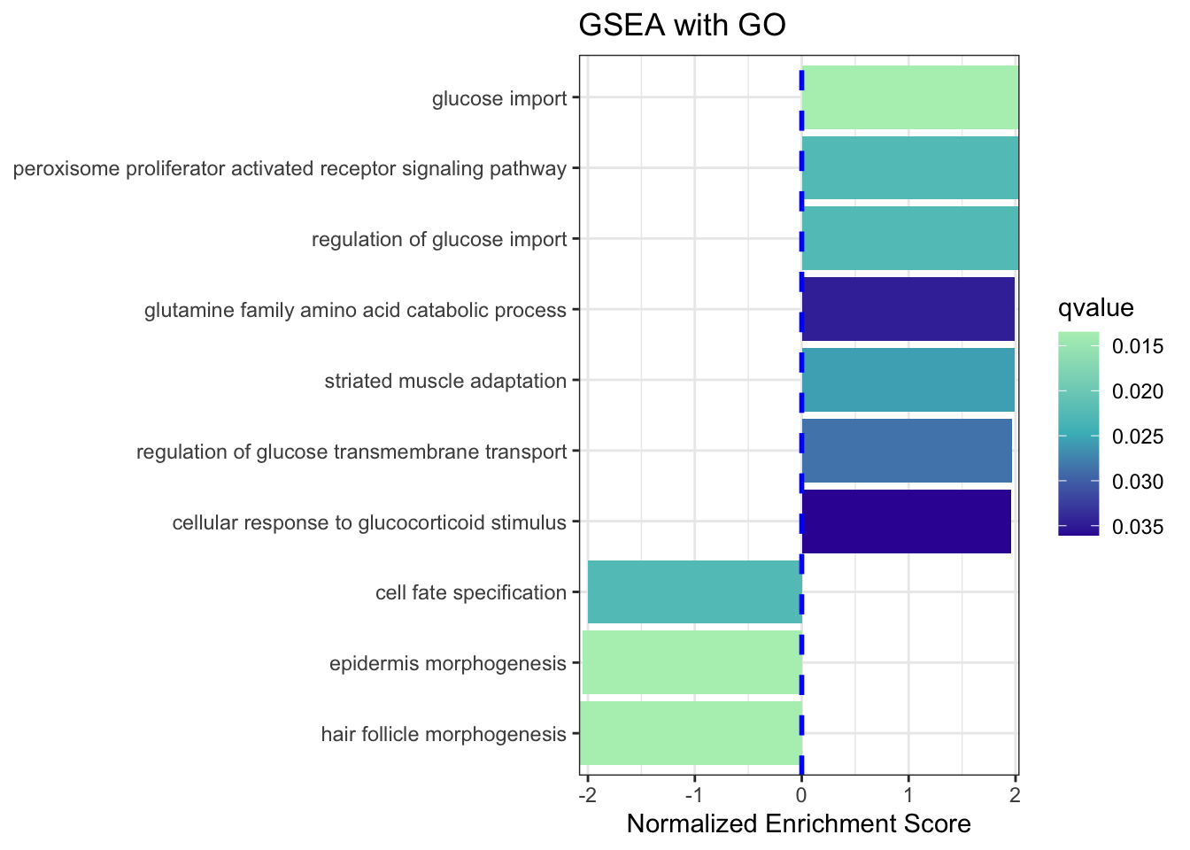
Let's filter the gseaResult to only include NES results greater than 1.95 or less than -2.
#filter
gsea_go2 <- filter(gsea_go,NES > 1.95 | NES < -2)
dim(gsea_go2)
[1] 10 11
#replot upset plot
enrichplot::upsetplot(gsea_go2,n=10)

#plot using a barplot
ggplot(gsea_go2, showCategory=10, aes(NES, fct_reorder(Description, NES),
fill=qvalue)) +
  geom_col() +
  geom_vline(xintercept=0, linetype="dashed", color="blue",size=1)+
  scale_fill_gradientn(colours=c("#b3eebe","#46bac2", "#371ea3"),
                       guide=guide_colorbar(reverse=TRUE))+
  scale_x_continuous(expand=c(0,0))+
  theme_bw() +
  #theme(text=element_text(size=8))+
  xlab("Normalized Enrichment Score") +
  ylab(NULL) +
  ggtitle("GSEA with GO")
Warning: Using `size` aesthetic for lines was deprecated in ggplot2 3.4.0.
ℹ Please use `linewidth` instead.
ChIPseeker
Following ChIP-seq, ChIPseeker paired with clusterProfiler can be used to connect functional analysis with genomic ROIs. See the vignette here.
Other packages to check out
GSVA package - useful for clinical data (large patient cohort).
pathview.
gProfileR.
Additional Resources
Readings
- Chicco D, Agapito G (2022) Nine quick tips for pathway enrichment analysis. PLoS Comput Biol 18(8): e1010348. https://doi.org/10.1371/journal.pcbi.1010348.
- Wijesooriya K, Jadaan SA, Perera KL, Kaur T, Ziemann M. Urgent need for consistent standards in functional enrichment analysis. PLoS Comput Biol. 2022 Mar 9;18(3):e1009935. doi: 10.1371/journal.pcbi.1009935. PMID: 35263338; PMCID: PMC8936487..
- Ludwig Geistlinger, Gergely Csaba, Mara Santarelli, Marcel Ramos, Lucas Schiffer, Nitesh Turaga, Charity Law, Sean Davis, Vincent Carey, Martin Morgan, Ralf Zimmer, Levi Waldron, Toward a gold standard for benchmarking gene set enrichment analysis, Briefings in Bioinformatics, Volume 22, Issue 1, January 2021, Pages 545–556, https://doi.org/10.1093/bib/bbz158
Useful tutorials
- Functional Analysis for RNA-seq: Over-representation Analysis
- Functional Analysis for RNA-seq: Functional Class Scoring
- Functional Enrichment Analysis.
R Session info
sessionInfo()
R version 4.2.3 (2023-03-15)
Platform: x86_64-apple-darwin17.0 (64-bit)
Running under: macOS Big Sur ... 10.16

Matrix products: default
BLAS:   /Library/Frameworks/R.framework/Versions/4.2/Resources/lib/libRblas.0.dylib
LAPACK: /Library/Frameworks/R.framework/Versions/4.2/Resources/lib/libRlapack.dylib

locale:
[1] en_US.UTF-8/en_US.UTF-8/en_US.UTF-8/C/en_US.UTF-8/en_US.UTF-8

attached base packages:
[1] stats4    stats     graphics  grDevices utils     datasets  methods
[8] base

other attached packages:
 [1] enrichplot_1.18.4     ReactomePA_1.42.0     DOSE_3.24.2
 [4] lubridate_1.9.2       forcats_1.0.0         stringr_1.5.0
 [7] dplyr_1.1.2           purrr_1.0.1           readr_2.1.4
[10] tidyr_1.3.0           tibble_3.2.1          ggplot2_3.4.2
[13] tidyverse_2.0.0       org.Hs.eg.db_3.16.0   AnnotationDbi_1.60.2
[16] IRanges_2.32.0        S4Vectors_0.36.2      Biobase_2.58.0
[19] BiocGenerics_0.44.0   clusterProfiler_4.6.2

loaded via a namespace (and not attached):
  [1] ggnewscale_0.4.8       fgsea_1.24.0           colorspace_2.1-0
  [4] ggtree_3.6.2           gson_0.1.0             qvalue_2.30.0
  [7] XVector_0.38.0         aplot_0.1.10           rstudioapi_0.14
 [10] farver_2.1.1           graphlayouts_1.0.0     ggrepel_0.9.3
 [13] bit64_4.0.5            fansi_1.0.4            scatterpie_0.1.9
 [16] codetools_0.2-19       splines_4.2.3          cachem_1.0.7
 [19] GOSemSim_2.24.0        knitr_1.42             polyclip_1.10-4
 [22] jsonlite_1.8.4         GO.db_3.16.0           png_0.1-8
 [25] graph_1.76.0           graphite_1.44.0        ggforce_0.4.1
 [28] compiler_4.2.3         httr_1.4.5             Matrix_1.5-4
 [31] fastmap_1.1.1          lazyeval_0.2.2         cli_3.6.1
 [34] tweenr_2.0.2           htmltools_0.5.5        tools_4.2.3
 [37] igraph_1.4.2           gtable_0.3.3           glue_1.6.2
 [40] GenomeInfoDbData_1.2.9 reshape2_1.4.4         rappdirs_0.3.3
 [43] fastmatch_1.1-3        Rcpp_1.0.10            vctrs_0.6.2
 [46] Biostrings_2.66.0      ape_5.7-1              nlme_3.1-162
 [49] ggraph_2.1.0           xfun_0.39              timechange_0.2.0
 [52] lifecycle_1.0.3        zlibbioc_1.44.0        MASS_7.3-59
 [55] scales_1.2.1           tidygraph_1.2.3        reactome.db_1.82.0
 [58] hms_1.1.3              ggupset_0.3.0          parallel_4.2.3
 [61] RColorBrewer_1.1-3     yaml_2.3.7             memoise_2.0.1
 [64] gridExtra_2.3          downloader_0.4         ggfun_0.0.9
 [67] HDO.db_0.99.1          yulab.utils_0.0.6      stringi_1.7.12
 [70] RSQLite_2.3.1          tidytree_0.4.2         BiocParallel_1.32.6
 [73] GenomeInfoDb_1.34.9    rlang_1.1.0            pkgconfig_2.0.3
 [76] bitops_1.0-7           evaluate_0.20          lattice_0.21-8
 [79] labeling_0.4.2         treeio_1.22.0          patchwork_1.1.2
 [82] htmlwidgets_1.6.2      cowplot_1.1.1          shadowtext_0.1.2
 [85] bit_4.0.5              tidyselect_1.2.0       plyr_1.8.8
 [88] magrittr_2.0.3         R6_2.5.1               generics_0.1.3
 [91] DBI_1.1.3              pillar_1.9.0           withr_2.5.0
 [94] KEGGREST_1.38.0        RCurl_1.98-1.12        crayon_1.5.2
 [97] utf8_1.2.3             tzdb_0.3.0             rmarkdown_2.21
[100] viridis_0.6.2          grid_4.2.3             data.table_1.14.8
[103] blob_1.2.4             digest_0.6.31          gridGraphics_0.5-1
[106] munsell_0.5.0          viridisLite_0.4.1      ggplotify_0.1.0