Lesson5: Visualizing clusters with heatmap and dendrogram
The following questions will help you gain more confidence in exploring data through heatmap. We will work with a subset of the Human Brain Reference (HBR) and Universal Human Reference (UHR) RNA sequencing dataset and use the heatmap to
- Visualize gene expression
- Determine whether subsets of genes can help us differentiate between the HBR and UHR samples
Load necessary packages
library(pheatmap)
library(tidyverse)
## ── Attaching packages ─────────────────────────────────────── tidyverse 1.3.2 ──
## ✔ ggplot2 3.3.6     ✔ purrr   0.3.4
## ✔ tibble  3.1.8     ✔ dplyr   1.0.9
## ✔ tidyr   1.2.0     ✔ stringr 1.4.0
## ✔ readr   2.1.2     ✔ forcats 0.5.1
## ── Conflicts ────────────────────────────────────────── tidyverse_conflicts() ──
## ✖ dplyr::filter() masks stats::filter()
## ✖ dplyr::lag()    masks stats::lag()
Question 1
Could you import the hbr_uhr_normalized_counts.csv file into your workspace?
Solution
hbr_uhr_normalized_counts <- read.csv("./data/hbr_uhr_normalized_counts.csv",row.names=1)
Question 2
Explore this gene expression dataset a bit. How many samples (columns) and genes (row names) does this dataset have?
Solution
This dataset contains 6 samples (
- HBR_1.bam
- HBR_2.bam
- HBR_3.bam
- UHR_1.bam
- UHR_2.bam
- UHR_3.bam
The samples with names starting with HBR are from the Human Brain Reference (HBR) and those with names starting with UHR are from the Universal Human Reference (UHR). Remember this for a later questions.
hbr_uhr_normalized_counts
##               HBR_1.bam HBR_2.bam HBR_3.bam UHR_1.bam UHR_2.bam UHR_3.bam
## SULT4A1           375.0     343.6     339.4       3.5       6.9       2.6
## MPPED1            157.8     158.4     162.6       0.7       3.0       2.6
## PRAME               0.0       0.0       0.0     568.9     467.3     519.2
## IGLC2               0.0       0.0       0.0     488.6     498.0     457.5
## IGLC3               0.0       0.0       0.0     809.7     313.8     688.0
## CDC45               2.6       1.0       0.0     155.0     152.5     149.9
## CLDN5              77.6      88.5      67.2       1.4       2.0       0.0
## PCAT14              0.0       0.0       1.2     139.8     154.4     155.1
## RP5-1119A7.17      53.0      57.6      51.9       0.0       0.0       0.0
## MYO18B              0.0       0.0       0.0      59.5      84.2      56.5
## RP3-323A16.1        0.0       0.0       1.2      51.9      76.2      53.1
## CACNG2             42.7      35.0      56.6       0.0       1.0       0.0
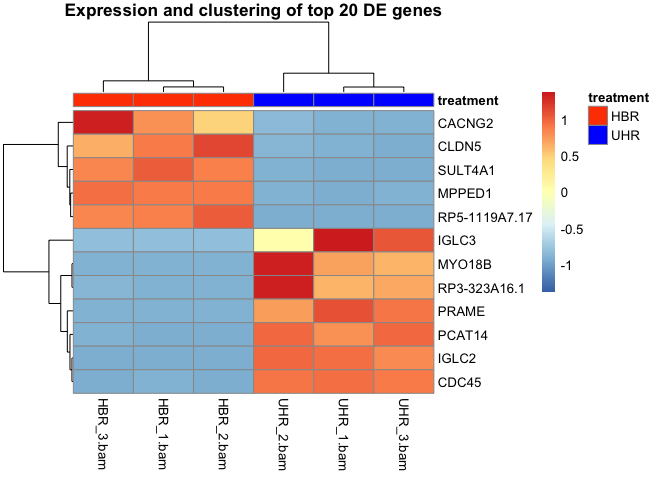
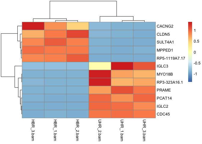
Question 3
Create a heatmap for to visualize gene expression for this dataset.
Solution
pheatmap(hbr_uhr_normalized_counts,scale="row")
Question 4
Create a data frame called annotation_df that contains the sample and treatment group information that we will add to the legend for this heatmap.
Solution
annotation_df <- data.frame(sample=c("HBR_1.bam","HBR_2.bam","HBR_3.bam","UHR_1.bam","UHR_2.bam","UHR_3.bam"),treatment=c(rep("HBR",3),rep("UHR",3))) %>% column_to_rownames("sample")
annotation_df
##           treatment
## HBR_1.bam       HBR
## HBR_2.bam       HBR
## HBR_3.bam       HBR
## UHR_1.bam       UHR
## UHR_2.bam       UHR
## UHR_3.bam       UHR
Question 5
Add the annotations for the legend and color the HBR samples orangered and the UHR samples blue. Also, add a title to the heatmap.
Solution
pheatmap(hbr_uhr_normalized_counts,scale="row", annotation_col =annotation_df,
         annotation_colors =list(treatment=c(HBR="orangered",UHR="blue")),
         main="Expression and clustering of top 12 DE genes")