Lesson 15: Finding differentially expressed genes
Before getting started, remember to be signed on to the DNAnexus GOLD environment.
Lesson 14 review
In the previous lesson, we learned to visualize RNA sequencing alignment results in the Integrative Genome Viewer (IGV).
Learning objectives
In this lesson, we will identify genes that are differentially expressed between conditions. Here, we want to compare UHR samples to HBR samples, so we will be using existing applications to determine the ratio of expression of genes in the UHR samples versus the HBR samples (ie. UHR / HBR) and then we will get a metric to determine whether the expression change is statistically significant. Below are the two tasks for this lesson.
- Get expression counts for genes in the Human Brain Reference (HBR) and Universal Human Reference (UHR) dataset
- Complete our analysis of the HBR and UHR data by obtaining genes that are differentially expressed between the two groups
- Visualize gene expression
Before getting started, make sure that we are in the ~/biostar_class/hbr_uhr directory.
cd ~/biostar_class/hbr_uhr
Obtaining expression read counts from alignment results
Let's talk about obtaining expression read counts using an application called featureCounts
First let's create a new directory in our ~biostar_class/hbr_uhr folder to store the counts.
mkdir hbr_uhr_deg_chr22
Next, change into the ~biostar_class/hbr_uhr_hisat2 folder
cd ~/biostar_class/hbr_uhr/hbr_uhr_hisat2
To run featureCounts we type in featureCounts at the command line followed by
- -p, specifies we want to count in the paired end mode since we are working with paired end sequencing
- -a, which prompts us to provide the annotation file (22.gtf)
- -g, which prompts us to specify attribute type in the GTF file (we choose to use gene_names so we can get expression by gene)
- -o prompts us to provide the output name
- finally, our input BAM files are provided
featureCounts -p -a ../refs/22.gtf -g gene_name -o ../hbr_uhr_deg_chr22/hbr_uhr_chr22_counts.txt HBR_1.bam HBR_2.bam HBR_3.bam UHR_1.bam UHR_2.bam UHR_3.bam
After featureCounts finishes, we can go into the hbr_uhr_deg_chr22 directory to see what we have.
cd ~/biostar_class/hbr_uhr/hbr_uhr_deg_chr22
ls -1
We have a file hbr_uhr_chr22_counts.txt with the expression counts and a summary. We will need the expression counts (ie. hbr_uhr_chr22_counts.txt) for differential expression analysis.
hbr_uhr_chr22_counts.txt
hbr_uhr_chr22_counts.txt.summary
If we take a look at the first two lines of hbr_uhr_chr22_counts.txt, we will see that featureCounts saves program information and command line call in the first line (we need to remove this line). The second line are the column headers. In the column headers, we do not need columns Chr, Start, End, Strand, and Length. All we want are the genes and expression for these genes in our samples.
head -2 hbr_uhr_chr22_counts.txt
# Program:featureCounts v2.0.1; Command:"featureCounts" "-a" "../refs/22.gtf" "-g" "gene_name" "-o" "../hbr_uhr_deg_chr22/hbr_uhr_chr22_counts.txt" "HBR_1.bam" "HBR_2.bam" "HBR_3.bam" "UHR_1.bam" "UHR_2.bam""UHR_3.bam"
Geneid  Chr     Start   End     Strand  Length  HBR_1.bam       HBR_2.bam       HBR_3.bam       UHR_1.bam       UHR_2.bam       UHR_3.bam
To remove the header line, we use the sed command below, where
- the option 1d indicates delete the first line (1 refers to the first line, d denotes delete)
- next we provide the input file
- we use ">" to indicate we want to save the output and then provide a name for the output (we will append "_no_header" to the original file name)
sed '1d' hbr_uhr_chr22_counts.txt > hbr_uhr_chr22_counts_no_header.txt
If we look at the first two rows of hbr_uhr_chr22_counts_no_header.txt, we should see the column headings and counts for the first gene. We still need to remove the columns Chr, Start, End, Strand, and Length. We will keep hbr_uhr_chr22_counts_no_header.txt because we need it for a downstream task.
head -2 hbr_uhr_chr22_counts_no_header.txt
Geneid  Chr     Start   End     Strand  Length  HBR_1.bam       HBR_2.bam       HBR_3.bam       UHR_1.bam       UHR_2.bam       UHR_3.bam
U2      chr22   10736171        10736283        -       113     0       0       0       0       0       0
To remove the columns Chr, Start, End, Strand, and Length, we can use cut
- where -f1,7-12 tells the command that we want field 1 (the gene ids) and then fields 7-12, the expression counts for the samples
- the output from cut is then piped to tr '\t' ',', which will replace the original tab ('\t') separated columns with comma (',') separated columns. In other words, rather than using tabs to separate the columns of our counts table, we use commas, which is required for the differential expression analysis software. We can do tr ',' '\t' to go from comma separated columns to tab separated columns
- we save the new counts table as counts.csv
cut -f1,7-12 hbr_uhr_chr22_counts_no_header.txt | tr '\t' ',' > counts.csv
Now, we can use the column command to look at the HBR and UHR expression counts table. Hit q to exit the column command and return to the terminal.
- -t: identifies the number of columns in the input
- -s: tells column command that the columns in the input are separated by commas
- |: pipe or sends the output of column to less -S where -S allows us to scroll to see columns of the table that would not fit on the terminal
column -t -s ',' counts.csv | less -S
Geneid              HBR_1.bam  HBR_2.bam  HBR_3.bam  UHR_1.bam  UHR_2.bam  UHR_3.bam
U2                  0          0          0          0          0          0
CU459211.1          0          0          0          0          0          0
CU104787.1          0          0          0          0          0          0
BAGE5               0          0          0          0          0          0
Normalization
Before diving into differential expression analysis, it is important to take a brief look at the concept of normalization. After obtaining expression counts, we will need to normalize the counts before performing differential expression analysis. This is an important step because normalization serves to remove technical variations amongst the samples to ensure that whatever difference we get in gene expression is due to biology.
Common sources of technical noise include the following and we would like to have them removed before continuing on with analysis.
- Differences in library size between the samples (ie. the sum of the counts between the samples are not the same). To understand this a bit better, think of a Western blot, where we have to load the same amount of protein or starting material (from each sample) into each lane in a gel so that we can compare protein expression.
- Gene length - the longer the gene the more reads it will get.
- Batch effect - when we process different samples on different days, locations, by different people etc. we are introducing technical noise.
While there are different approaches for normalization, we will not explore these today as it is a more advanced topic. Also, some of the differential expression analysis packages such as DESeq2 and edgeR have their own normalization procedures and users are instructed to input only the raw integer counts when using these packages.
For now, we will use scripts written by the author of the Biostars handbook. These scripts can be run on the command line but they are R packages, so for those interested in learning R, please visit https://bioinformatics.ccr.cancer.gov/btep/classes/ for our series of introductory R courses.
Differential expression analysis
Prior to differential expression analysis, we need to generate a design.csv file that contains the samples and their corresponding treatment conditions. Note that csv stands for comma separated value so the columns in these files are separated by commas. This file is already created for us and it lives in the design_file_hisat2 folder, which we should see in our home directory.
If we listed the contents of the design_file_hisat2 folder, we will see two files
ls ~/design_file_hisat2
design.csv design.txt
Copy both files (design.csv and design.txt) to the ~/biostar_class/hbr_uhr/hbr_uhr_deg_chr22 folder, which should be the present working directory.
cp ~/design_file_hisat2/design.csv .
cp ~/design_file_hisat2/design.txt .
We will need the design.txt file when we do visualizations.
The design.csv file and design.txt file contain the same content, except the columns in the csv file are separated by commas and the txt file are separated by tabs. We can use cat to view these.
cat design.csv
sample,condition
HBR_1.bam,HBR
HBR_2.bam,HBR
HBR_3.bam,HBR
UHR_1.bam,UHR
UHR_2.bam,UHR
UHR_3.bam,UHR
cat design.txt
sample  condition
HBR_1.bam       HBR
HBR_2.bam       HBR
HBR_3.bam       HBR
UHR_1.bam       UHR
UHR_2.bam       UHR
UHR_3.bam       UHR
To get differential expression for genes on chromosome 22, we will need make sure we are in ~/biostar_class/hbr_uhr/hbr_uhr_deg_chr22 folder (use pwd to confirm and cd into if needed) and run the deseq2.r script as shown below.
Rscript $CODE/deseq2.r
While the deseq2.r script is running, it will generate the following. Mainly, it's telling us that it is using the design.csv and counts.csv files as input and the output is stored in results.csv.
converting counts to integer mode
estimating size factors
estimating dispersions
gene-wise dispersion estimates
mean-dispersion relationship
final dispersion estimates
fitting model and testing
[1] "# Tool: DESeq2"
[1] "# Design:  design.csv"
[1] "# Input:  counts.csv"
[1] "# Output:  results.csv"
Since the differential analysis results are in csv format, we can open these in Excel. However, we can also view these in the terminal using the column command. And doing this we find that there are 13 columns in the differential analysis results table and they are described below. Hit q to get out of the column command.
column -t -s ',' results.csv | less -S
- name: gene names.
- baseMean: average expression across all samples (HBR+UHR).
- baseMeanA: average expression across samples of treatment group A (HBR in this case).
- baseMeanB: average expression across samples of treatment group B (UHR in this case).
- foldChange: ratio of expression between UHR and HBR (ie. baseMeanB/baseMeanA)
- log2FoldChange: log2 of the values in the foldChange column, this scales our fold change results uniformly. A fold change of 2 corresponds to a log2 fold change of 1, while a fold change of 1/2 corresponds to a log2 fold change of -1
- lfcSE is the standard error of the log2 fold change.
- stat: our test statistics, which is obtained by log2FoldChange/lfcSE and is used to derive the statistical significance.
- PValue: the uncorrected p-value of the likelihood of observing the effect of the size foldChange (or larger) by chance alone. This p-value is not corrected for multiple comparisons.
- PAdj: Multiple comparison adjusted p-value.
- FDR: the False Discovery Rate - this column represents the fraction of false discoveries for all the rows above the row where the value is listed. For example, if in row number 300 the FDR is 0.05, it means that if you cut the table at this row and accept all genes at and above it as differentially expressed then, 300 * 0.05 = 15 genes out of the 300 are likely to be false positives. The values in this column are also called q-values.
- falsePos: this column is derived directly from FDR and represent the number of false positives in the rows above.
- The last six columns are normalized expression for each of the samples.
We can use the command below to sort by log2 fold change from largest to smallest, where
- column is used to print our tabular data nicely with columns aligned
- -t indicates to separate the columns by a tab
- -s ',' indicates that the columns in our file are originally separated by comma (ie. a csv file)
- sed 1q will print the first line of our table and then quits, preventing the first line from being included in the sort
- we use sort to sort things
- -k: prompts us to provide column that we want to sort by, here it is column 6 (log2 fold change),
- n indicates we want to sort numerically
- r indicates in reverse order (from largest to smallest)
Hit q to exit and return to prompt
column -t -s ',' results.csv | (sed 1q; sort -k6nr) | less -S
name                baseMean  baseMeanA  baseMeanB  foldChange  log2FoldChange  lfcSE  stat    PValue    PAdj      FDR     falsePos  HBR_1.bam  HBR_2.bam  HBR_3.bam  UHR_1.bam  UHR_2.bam  UHR_3.bam
PRAME               521.8     0          1043.6     4883.081    12.3            1.18   10.36   3.9e-25   3.6e-22   0       0         0          0          0          1144.9     946.2      1039.7
IGLC2               485.9     0          971.8      4538.584    12.1            1.19   10.25   1.2e-24   1.1e-21   0       0         0          0          0          937.4      1142.1     835.9
IGLC3               386.2     0          772.5      3616.649    11.8            1.19   9.94    2.8e-23   2.6e-20   0       0         0          0          0          945.1      572.6      799.8
MYO18B              63.8      0          127.7      595.615     9.2             1.22   7.57    3.7e-14   3.2e-11   0       0         0          0          0          113.9      162.6      106.6
PCAT14              145.5     0.8        290.3      375.805     8.6             1.04   8.24    1.7e-16   1.5e-13   0       0         0          0          2.4        270.3      296.9      303.6
CDC45               149.4     1.5        297.2      192.61      7.6             0.75   10.19   2.3e-24   2.1e-21   0       0         2.6        2          0          300.4      297.9      293.3
RP3-323A16.1        61        0.8        121.2      156.473     7.3             1.07   6.83    8.2e-12   7.0e-09   0       0         0          0          2.4        103.4      153.5      106.6
ZNF280A             10.1      0          20.3       94.53       6.6             1.39   4.74    2.2e-06   1.8e-03   0       0         0          0          0          15.4       22.2       23.2
Visualizing differential expression results
Plots condense complex and busy tabular data into a form that is easier to interpret. An expression heatmap is a common visualization used in RNA sequencing analysis. A heatmap shows numerical data on a color scale and is often combined with a dendrogram that shows how groups cluster. Here, we will generate an expression heatmap for HBR and UHR dataset using the script create_heatmap.r. The input for the script is results.csv, containing our differential gene expression findings generated by the deseq2.r script.
Rscript $CODE/create_heatmap.r
To view the expression heatmap, copy it to ~/public. Go back to the GOLD landing page, click on the "Files" tab associated with your name and you will be taken to an index page. You can click on PDF files and view in them in the browser without having to download them.
cp heatmap.pdf ~/public/heatmap_hisat2.pdf
Figure 1 shows the expression heatmap for the chromosome 22 genes in the HBR and UHR samples. On the top of the plot, we have a color key, which indicates that down regulated genes have negative values and these are colored by shades of green and up regulated genes have positive values and these are colored by shades of red. The horizontal axis of the heatmap are labeled with the sample names, the right vertical axis are the genes, the left vertical axis is the dendrogram that shows clustering of genes based on expression. In this expression heatmap, it is clear that there are gene clusters that are up regulated or down regulated in one group but not the other.

Figure 1
Another common visualization in RNA sequencing is Principal Component Analysis (PCA) plot. This helps us visualize clusters of samples in our data by transforming our data so that we can visualize along the axes that capture the largest variation in the data. We will use the creat_pca.r script and the command below to generate our PCA. The input for this script is our counts table (counts.csv) but we need a tab separated version of it. We also need design.txt (tab separated version of the design file) and the number of samples we have (6 in the case of the HBR and UHR dataset).
First use cat and tr to create tab separated counts table from counts.csv. The tr command replaces ',' with tabs ('\t').
cat counts.csv | tr ',' '\t' > counts.txt
Then, we run the R script create_pca.r where the inputs are counts.txt (tab separated expression counts table), design.txt, and 6 (the number of samples).
Rscript $CODE/create_pca.r counts.txt design.txt 6
To view the PCA, copy it to ~/public.
cp pca.pdf ~/public/pca_hisat2.pdf
The PCA plot is shown in Figure 2. The HBR samples are colored in red dots and UHR samples are colored in the green dots. The horizontal axis (PC1) is the one that captures the most variance or separation (79%) in our samples. PC2 on the vertical axis captures the second most variance or separation (7%). We see that along PC1, the HBR and UHR samples are clearly separated and we are able to see perhaps the biological difference between these samples. Along PC2, while the HBR samples cluster closely, we see that the UHR_2 sample is off by itself (away from the other two samples in this group). This could indicate some underlying biology of UHR_2 or maybe it's caused by some technical factor.
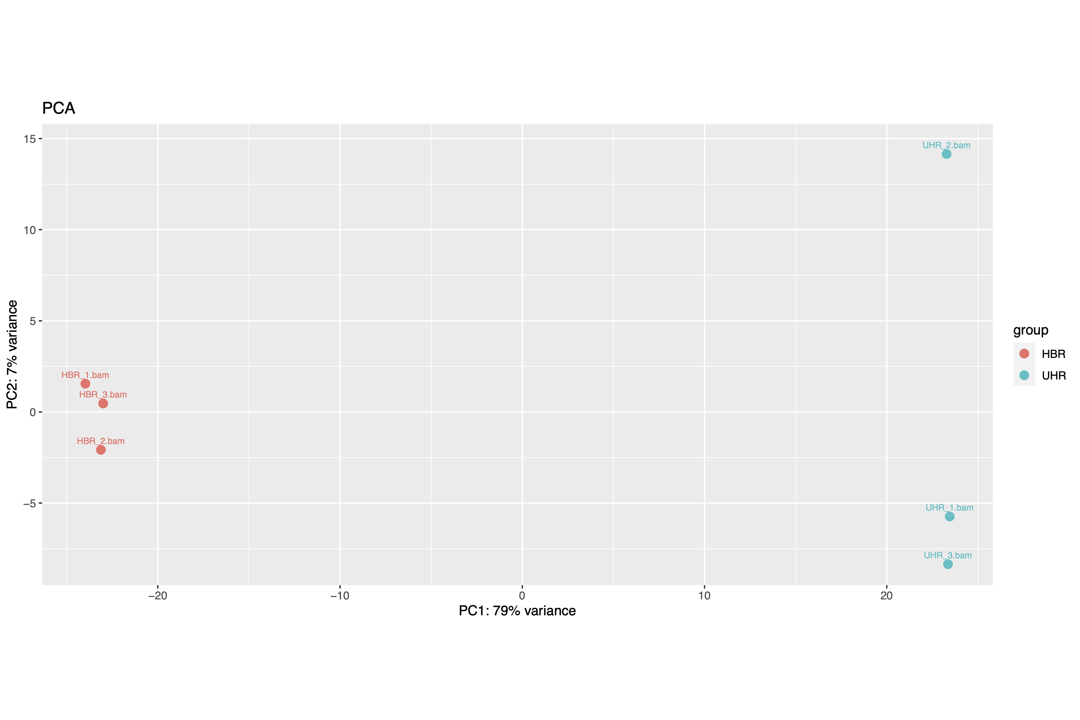
Figure 2