Lesson 9: Reference genomes and genome annotations used in RNA sequencing
Before getting started, remember to be signed on to the DNAnexus GOLD environment.
Lesson 8 Review
In Lesson 8, we learned about the basics of RNA sequencing, including experimental considerations and basic ideas behind data analysis. In lessons 9 through 17 we will learn how to analyze RNA sequencing data. We will start with quality assessment, followed by alignment to a reference genome, and finally identify differentially expressed genes.
Learning Objectives
In this lesson, we will continue to learn about RNA sequencing analysis using the Human Brain Reference (HBR) and Universal Human Reference (UHR) datasets. In particular, we will
- Get to know the HBR and UHR dataset
- Locate the data and analysis tools
- Introduce the reference genomes
- Provide a brief introduction to the Integrative Genome Viewer( IGV) - to focus on visualizing the reference genome and genomic features
About the Human Brain Reference and Universal Human Reference data
The Human Brain Reference (HBR) RNA sequencing data are derived from RNA extracted from
- 23 human brains
- brains are from both males and females, age ranging from 60 to 80 years
The Universal Human Reference data used RNA from 10 cancer cell lines.
These two experiments used the External RNA Control Consortium (ERCC) spike-in RNAs as controls. These internal standards provide a known quantity of RNA to evaluate the quality of RNA sequencing experiment. They can provide information on dynamic range, limits of detection, and reliability of differential expression results. To learn more about ERCC spike-ins refer to the following:
- https://www.thermofisher.com/order/catalog/product/4456740
- https://www.nist.gov/programs-projects/external-rna-controls-consortium
- ERCC seminar
- ERCC publication
- ERCC Bioconductor package
Where is my data?
Here, let's download the HBR and UHR dataset to get acquainted with it.
First, we will use pwd to make sure we are in the home directory.
pwd
If we are in the home directory, we will see the following output displayed in the terminal where "username" is your username, or student id that you used to sign into the terminal.
/home/usernanme
If not in the home directory use the command below to get back.
cd
Then create a folder called biostar_class and change into this folder.
mkdir biostar_class
cd biostar_class
Let's keep the analysis results of the HBR and UHR dataset to a folder called hbr_uhr, so we need to create this and then change into it.
mkdir hbr_uhr
cd hbr_uhr
Now it's time to download the HBR and UHR dataset. What are the two commands that we can use to download data from the web?
Solution
We can use curl OR wget to download data from the web.
Here, we will use wget to download the HBR and UHR dataset (remember, we should now be in the ~/biostar_class/hbr_uhr directory).
Using the wget command we just need to enter the command, which is wget, and then provide the URL to the file.
wget http://data.biostarhandbook.com/rnaseq/projects/griffith/griffith-data.tar.gz
If wget does not work, try curl. If using curl, we need to make sure to specify an output file name using the -o option.
curl http://data.biostarhandbook.com/rnaseq/projects/griffith/griffith-data.tar.gz -o griffith-data.tar.gz
If we now listed the content of the ~/biostar_class/hbr_uhr directory (recall that ~ denotes home directory), we will see the file griffith-data.tar.gz. Recall that this an archive of a collection of files that has been zipped (or compressed) to save on storage space.
ls
griffith-data.tar.gz
We can use the tar command to unpack the contents of griffith-data.tar.gz. In the tar command below, we include the following flags
- -x means - extract to disk from the tar (tape archive)
- -v means - produce verbose output. When using this flag tar will list each file name as it is read from the tar (tape archive), this allows us to see what is being extracted
- -f (file) means read the tar (tape archive) from or to the specified file
tar -xvf griffith-data.tar.gz
We do ls -l (where -l denotes list contents of a directory in the long view), we will see two additional folders
ls -1
-rw-rw-r-- 1 username username 131302475 Dec  5  2018 griffith-data.tar.gz
drwxrwxr-x 1 username username       264 Oct 19 17:27 reads
drwxrwxr-x 1 usernamels  username        60 Oct 19 17:27 refs
The sequencing reads for the HBR and UHR dataset reside in the reads directory. Below, we will list the content of the reads directory using ls -1 where -1 tells ls to list directory contents, but with one item per row. We will talk about these fastq or fq files later.
ls -1 reads
HBR_1_R1.fq
HBR_1_R2.fq
HBR_2_R1.fq
HBR_2_R2.fq
HBR_3_R1.fq
HBR_3_R2.fq
UHR_1_R1.fq
UHR_1_R2.fq
UHR_2_R1.fq
UHR_2_R2.fq
UHR_3_R1.fq
UHR_3_R2.fq
In this lesson, the focus is to get to know the reference genome and annotation files.
ls refs
In the refs folder, we have two fasta (fa) files. One is the reference genome for human chromosome 22 (see file 22.fa) and the other is the reference genome for ERCC spike-ins (see file ERCC92.fa). We will only be using 22.fa here.
We also have two gtf files that tells us about features that exist in a genome. Again, because we are not working with ERCC, we will ony be using the 22.gtf file, which tells us about the features that exist on human chromosome 22.
22.fa 22.gtf ERCC92.fa ERCC92.gtf
Where are the analysis tools?
Throughout this module, we will be running various tools, including helper R scripts on the Unix command line to analyze the HBR and UHR RNA sequencing dataset. The helper R scripts were developed by the author of the Biostars Handbook.
The tools include those used for
- Sequencing data quality assessment
- FASTQC
- MultiQC
- Quality and adapter trimming of sequencing data
- Trimmomatic
- BBDuk
- Alignment to genome or transcriptome
- HISAT2
- Salmon
- Obtain expression counts
- featureCounts
- combine_transcripts.r (R helper script used to combine count files from Salmon alignment)
- Differential expression analysis
- deseq2.r (R helper script)
- Visualize gene expression
- create_map.r (R helper script)
- create_pca.r (R helper scripts)
For the non-R based tools, we can run them at the command line. You can see a full list of non-R based tools if you listed the contents of the /miniconda3/bin folder although there is no need to go into this folder to do anything.
ls /miniconda3/bin
The R helper scripts are a bit different. They are located in the folder /usr/local/code.
ls -1 /usr/local/code
combine_genes.r
combine_transcripts.r
compare_results.r
create_heatmap.r
create_pca.r
create_tx2gene.r
deseq2.r
edger.r
filter_counts.r
mission-impossible.mk
parse_featurecounts.r
- The path to the R helper scripts, /usr/local/code, has been exported as the environmental variable CODE.
- If we ls $CODE, we should see the contents of the directory as well.
- This prevents us from typing a long path when running the R helper scripts.
- For example, if we wanted to use deseq2.r, we can type in the command line Rscript $CODE/deseq2.r
(Note we run the R helper scripts by starting off with the Rscript command.)
ls $CODE
The reference genome and annotation files
Now that we have downloaded the HBR and UHR dataset and know where analysis tools are, let's start learning about RNA sequencing, by first learning about our reference genome and annotation files. Let's stay in the ~/biostar_class/hbr_uhr/refs folder for this, if not then change into this directory.
cd ~/biostar_class/hbr_uhr/refs
We start off with the reference genome file (the .fa file) used for the HBR and UHR dataset, where the human chromosome 22 reference is derived from the GRCh38 version of the human reference genome.
To start, look at the content inside 22.fa by using head. View the first 3 lines (indicated by -3). A FASTA file can have extensions (.fasta or .fa).
head -3 22.fa
A "fasta" file contains nucleotide sequences. The first line is always a header or definition line that starts with ">".
>chr22
NNNNNNNNNNNNNNNNNNNNNNNNNNNNNNNNNNNNNNNNNNNNNNNNNNNNNNNNNNNN
NNNNNNNNNNNNNNNNNNNNNNNNNNNNNNNNNNNNNNNNNNNNNNNNNNNNNNNNNNNN
This definition line tells us information about the nucleotide sequence such as which chromosome is found (22 in our example as denoted by chr22). The first few lines of the chromosome 22 reference are N, where the nucleotide is unknown.
Note that the definition line can provide more information, depending on how the sequence was curated. As an example, in the human ADSL transcript nucleotide sequence, the header line tells us the accession number or sequence ID (NM_001363840.3), species in which the sequence was derived (Homo sapiens), name of the gene (ADSL), and that this is a mRNA sequence.
Below we use grep with the -v option so that it does not show any lines in the FASTA file that contains the search pattern (in this case N - the unknown nucleotides in this case) to see some actual sequences in chromosome 22, to make sure that the 22.fa file does contain meaningful sequences.
grep -v N 22.fa | head
>chr22
TAAGATGTCCTATAATTTCTGTTTGGAATATAAAATCAGCAACTAATATGTATTTTCAAA
GCATTATAAATACAGAGTGCTAAGTTACTTCACTGTGAAATGTAGTCATATAAAGAACAT
AATAATTATACTGGATTATTTTTAAATGGGCTGTCTAACATTATATTAAAAGGTTTCATC
AGTAATTCATTATATCAAAATGCTCCAGGCCAGGCGTGGTGGCTTATGCCTGTAATCCCA
GCACTTTGGGAGGTCGAAGTGGGCGGATCACTTGAGGTCAGGAGTTGGAGACTAGCCTGG
CCAACATGATGAAACCCCGTCTCTAATAATAATAATAAAAAAAAATTAGCTGGGTGTGGT
GGTGGGCAACTGTAATCTCAGCTAATCAGGAGGCTGAGGCAGAAGAATTGCTTGAACGTG
GAAGACAGAGTTTACAGTGTGCCAAGATCACACCACCCTACTCCAACTTGGGTGACAGAG
CAAGACTCAGTCTCAAGGAAAAAAAAAAGCTCGAAAAATGTTTGCTTATTTTGGTAAAAT
Here, we find that the human chromosome 22 reference (22.fa) is a file with a header or definition line with the nucleotide sequence of that entire chromosome. But what is it good for? 22.fa contains the known sequences of human chromosome 22, thus it's a reference that we can compare other sequences to. For high throughput sequencing, we need the known sequences so that we can find out where in the genome each of the sequencing reads came from. The reference genome in a way acts like a template that we can follow to reconstruct the genome of the unknown. In other words, think of the reference genome as a picture of the completed puzzle that helps us assemble the actual puzzle, by allowing us to overlap the pieces to see if they fit the completed version.
A question we might ask about the reference genome is how big is the reference (ie. how many bases)? To answer this, we can use the tool seqkit and it's stats feature.
Why do we need the size of the genome?
Prior to the sequencing experiment, the size of the genome will help us determine the number of reads needed to achieve a certain coverage (https://www.illumina.com/documents/products/technotes/technote_coverage_calculation.pdf).
After the experiment, we could use the size of our genome along with other information to decide the computing resources (ie. time and memory) needed for our analysis. Chromosome 22 is the second smallest in humans, so it would be faster to align to this than the entire human genome. For the sake of time in this class, that's why we chose to align to just this chromosome.
seqkit stats 22.fa
file   format  type  num_seqs     sum_len     min_len     avg_len     max_len
22.fa  FASTA   DNA          1  50,818,468  50,818,468  50,818,468  50,818,468
What is in the 22.gtf file? A gtf file is known as Genome Transfer File, which is essentially a tab delimited file (ie. columns in the file are separated by tab). It informs us of where different features such as genes, transcripts, exons, and coding sequences are found in a genome.
A gtf file is needed for couple of reasons.
First, even though we will map the RNA sequencing reads to a genome, we need to know which genomic features (ie. genes) the reads are aligning to generate some metric for expression (counts) and then perform differential expression analysis.
Second, because some of the sequencing reads can map to two exons, if we use a splice-aware-aligner, the information in the gtf file can be used to recognize the exon-exon boundaries (see Figure 1).
Otherwise, those reads that map to two exons will not be mapped and we end up losing information. See https://useast.ensembl.org/info/website/upload/gff.html for required information in a gtf file.
Table 2 shows the first three lines of 22.gtf.
The "score" column values represent the confidence in a feature existing in that genomic position. In this example the score contains a dot ".", which represents a missing value.
The frame column provides reading frame information. Where a "." appears in the gtf table, this means that the information is not available.
In Table 2, we are looking at gene ENSG00000277248.1, where the first line tells us that the feature is a gene, and the lines below this shows the transcript products for the gene as well as exons associated for that transcript.
Table 2: Preview of information presented in a gtf file
| CHROMOSOME | DATA SOURCE | FEATURE | START | END | SCORE | STRAND | FRAME | ATTRIBUTE |
|---|---|---|---|---|---|---|---|---|
| chr22 | ENSEMBL | gene | 10736171 | 10736283 | . | - | . | gene_id "ENSG00000277248.1"; gene_type "snRNA"; gene_status "NOVEL"; gene_name "U2"; level 3; |
| chr22 | ENSEMBL | transcript | 10736171 | 10736283 | . | - | . | gene_id "ENSG00000277248.1"; transcript_id "ENST00000615943.1"; gene_type "snRNA"; gene_status "NOVEL"; gene_name "U2"; transcript_type "snRNA"; transcript_status "NOVEL"; transcript_name "U2.14-201"; level 3; tag "basic"; transcript_support_level "NA"; |
| chr22 | ENSEMBL | exon | 10736171 | 10736283 | . | - | . | gene_id "ENSG00000277248.1"; transcript_id "ENST00000615943.1"; gene_type "snRNA"; gene_status "NOVEL"; gene_name "U2"; transcript_type "snRNA"; transcript_status "NOVEL"; transcript_name "U2.14-201"; exon_number 1; exon_id "ENSE00003736336.1"; level 3; tag "basic"; transcript_support_level "NA"; |
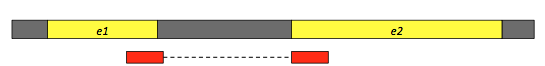
Figure 1: A sequencing read (red fragments) aligning two exons (e1 and e2). Modified from: https://training.galaxyproject.org/training-material/topics/transcriptomics/tutorials/rb-rnaseq/tutorial.html
To view the gtf or other tabular data in Unix, we can cat the file and then pipe or send the output to the column command, which allows us to print the columns so that they are nicely aligned. In this case, we use the -t option in column to determine the number of columns in the input and by default white space is used to separate the columns. Piping to less -S allows us to truncate some really long lines like those found in the attributes column of the gtf file and this also allows us to scroll horizontally to view additional columns. Hit Q to exit the cat command.
cat 22.gtf | column -t | less -S
chr22  ENSEMBL  gene            10736171  10736283  .  -  .  gene_id  "ENSG00000277248.1";   gene_type      "snRNA";                               gene_status  "NOVEL";                >
chr22  ENSEMBL  transcript      10736171  10736283  .  -  .  gene_id  "ENSG00000277248.1";   transcript_id  "ENST00000615943.1";                   gene_type    "snRNA";                >
chr22  ENSEMBL  exon            10736171  10736283  .  -  .  gene_id  "ENSG00000277248.1";   transcript_id  "ENST00000615943.1";                   gene_type    "snRNA";
Visualizing the reference genome and annotations
One of the things we will be doing quite often is to visualize genomics data using some sort of genome browser. In this course series, we will use a popular one called Integrative Genome Viewer(IGV). Let's visualize human chromosome 22 in IGV as a way to start becoming acquainted with the software.
Here, we will be using IGV that is installed on our local machine.
Instructions to install IGV:
Submit ticket to service.cancer.gov to get IGV installed on your machine.
We also need to download 22.fa and 22.gtf to our local desktop. To do this copy both into the ~/public directory.
cp 22.fa ~/public
cp 22.gtf ~/public
From there, download 22.fa and 22.gtf to our local machine. Note where the files were downloaded.
When we open IGV, we will see the window shown in (Figure 2).
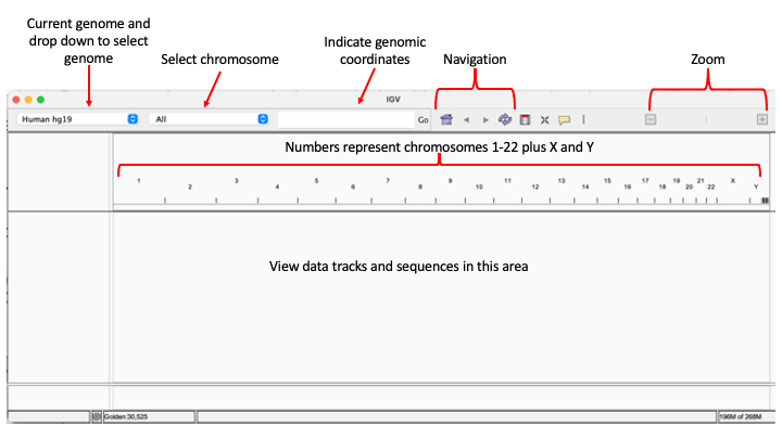
Figure 2
IGV comes preloaded with several genomes, but if we do not see the one we need in the drop down menu we can always load it from the Genomes drop down on the menu bar where it gives us some options including loading the genome from local file or from the web or URL (Figure 3). Compatible file formats include FASTA, JSON, or ".genome".

Figure 3:
To load data into IGV, we will choose one of the options in the File drop down in the menu bar (see Figure 4). Note that from the File drop down, we can take snap shots of our view and save as either PNG or SVG images.

Figure 4:
Since IGV loaded hg19 upon startup, we will load the chromosome 22 reference genome using the Load from File option under the Genomes drop down in the menu bar (Figure 5).
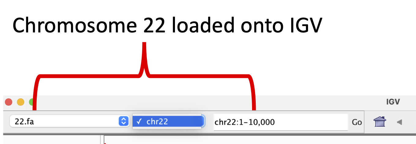
Figure 5:
Next, we will load the 22.gtf file onto IGV so we can see the genes aligned to the reference genome (Figure 6). The blue rectangles represent genes and transcripts, we can zoom in to look at ENSG00000280363.1 by searching for this gene ID in the Go box (we can actually search by coordinates, ID, or name).
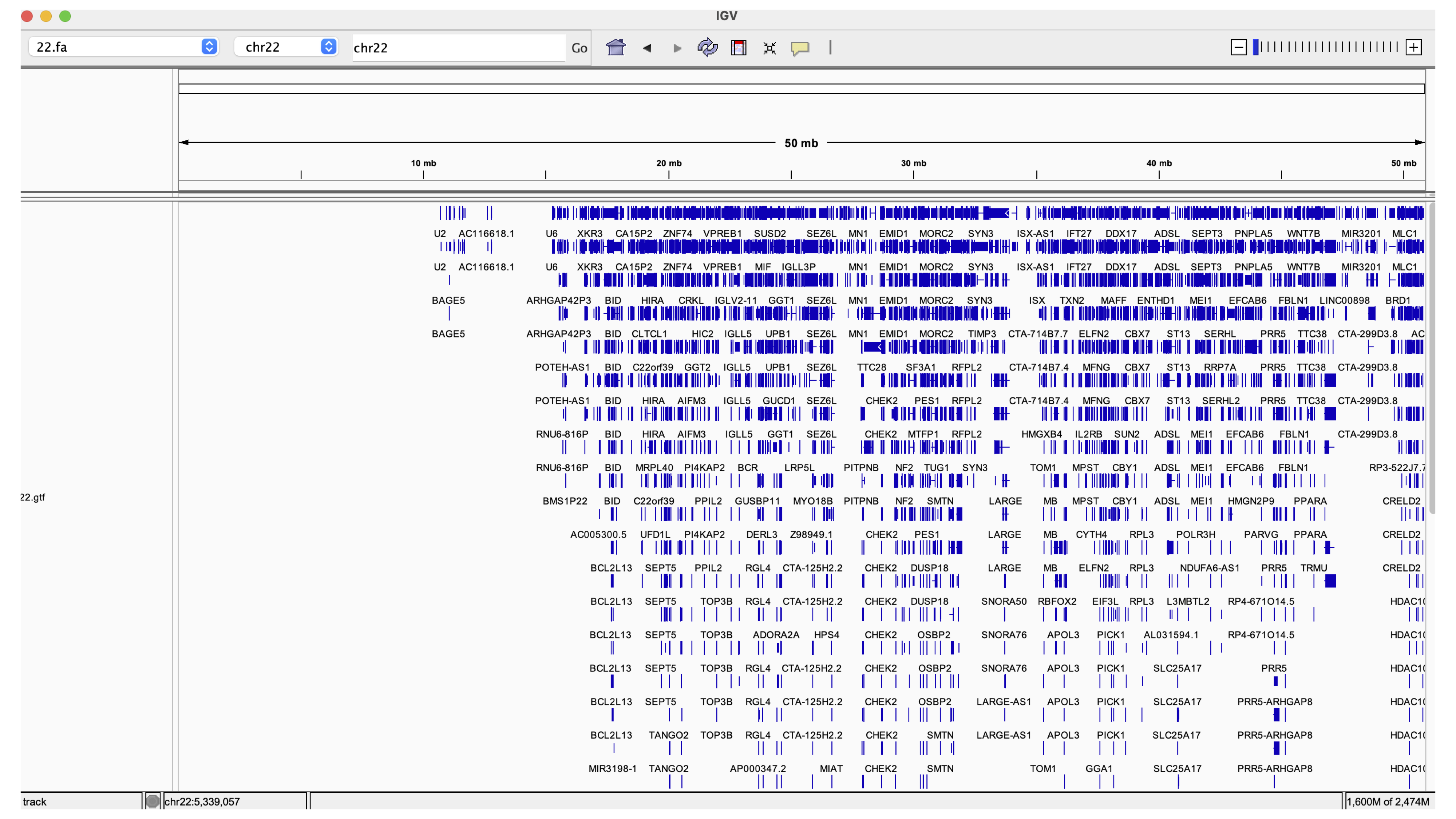
Figure 6
In Figure 7, we zoom into ENSG00000280363.1 on IGV, where ENSG00000280363.1 is the Ensembl accession number for gene CU104787.1. This gene overlaps ENSG00000279973.1, which is bage5. If we click on the solid blue line for each of the genes, a dialog box with more information will appear. The arrows on the genes point to the direction in which the gene was transcribed (these two genes were transcribed in different directions). Note that even though we search by gene ID in the Go box, the genomic coordinates will be displayed after IGV finds what we are looking for.
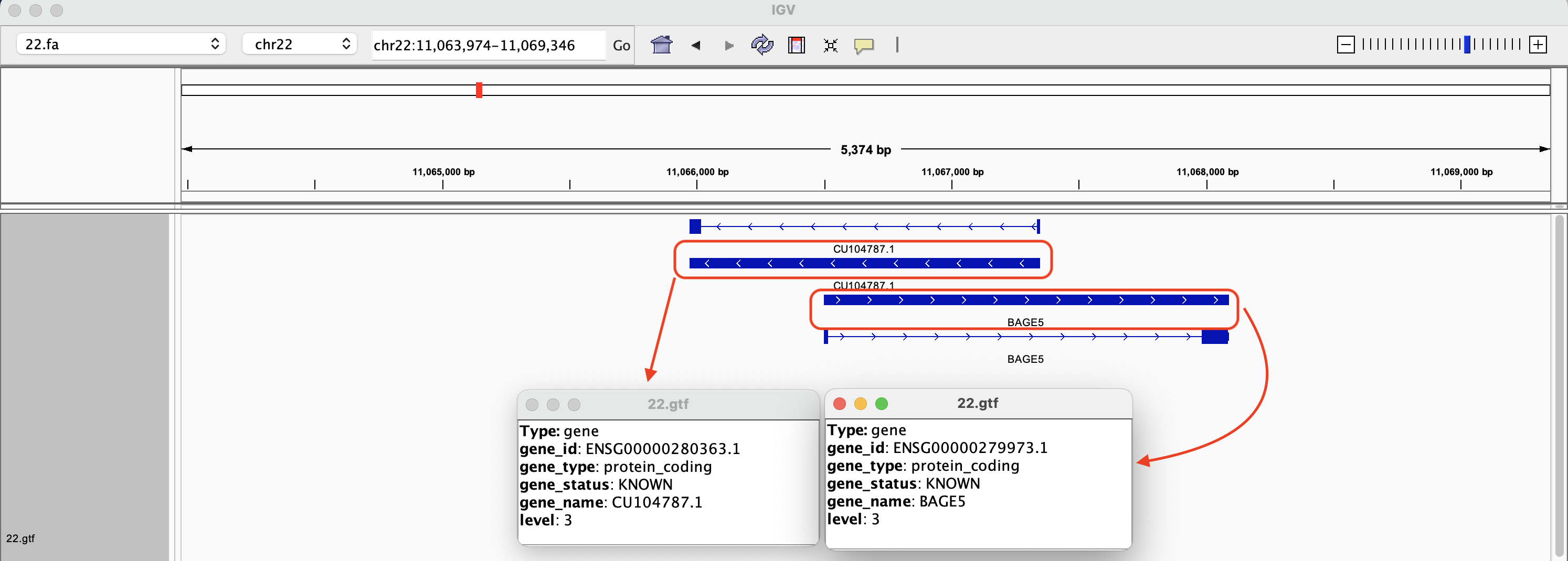
Figure 7
The transcripts are depicted by solid rectangles separated by lines (Figure 8). The solid rectangles are exons and the lines connecting are introns. If we click on the transcripts, a box pops up and we get more information regarding the transcript.
![]()
Figure 8
Within the exons, narrower solid rectangles represent untranslated regions or UTRs (Figure 9).

Figure 9
Among the many features of IGV, is the ability for users to zoom in close enough to see the bases (Figure 10).

Figure 10