Lesson 16: RNA sequencing review and classification based analysis
Before getting started, remember to be signed on to the DNAnexus GOLD environment.
Review
In the previous classes, we learned about the steps involved in RNA sequencing analysis. We started off with assessing quality of raw sequencing data, then we aligned the raw sequencing data to genome, and finally we obtained expression counts and conducted differential expression analysis.
Tools for assessing sequencing data quality
- FASTQC to obtain quality metrics for individual FASTQ files. Recall that FASTQ files contain our sequencing data and each file has many sequencing reads. Each read is composed of four lines
- Header, that starts with @
- Actual sequence
- "+"
- Quality, which tells us the error likelihood of the base call
- MultiQC to aggregate multiple FASTQC outputs into one
Tools for sequencing data cleanup
When analyzing high throughput sequencing data, we will need to trim away adapters. Adapters help anchor the unknown sequencing template to the Illumina flow cell and can interfere with alignment. We may also want to trim away low quality reads. In this course, we learned to use Trimmomatic, which is a flexible trimming tool for Illumina data to trim away low quality reads and adapters. Refer to the Trimmomatic manual and the Trimmomatic publication for details on how to use this tool.
Revisiting the construction of the trimmomatic command
- Initiate with the command by typing trimmomatic at the prompt
- Tell trimmomatic whether we are working with single end (SE) or paired end (PE) sequencing
- Provide input files
- Provide names of the output files including ones for unpaired reads (ie. those that survived the processing in one file but not the other)
-
Use SLIDINGWINDOW for quality trimming (see Figure 1)
- specify window size (ie. how many bases the sliding window is composed of), in the example below we use a window size of 4 bases
- specify the average quality score threshold for the window, in the example below we use 30
- in the example below, we will scan starting from the 5' end of the read, 4 bases at a time and trim once the average quality within a 4-base window falls below 30
-
ILLUMINACLIP is used to trim away adapters and other Illumina-specific sequences, the parameters needed for ILLUMINACLIP are
- FASTA file containing the adapter sequence
- some numbers indicating a threshold on how Trimmomatic will determine whether adapter is present in a read (to put these numbers in context, think of how BLAST works), in the example below we use 2, 30, and 5
- 2: seed mismatch threshold - "Specifies the maximum mismatch count which will still allow a full match to be performed. Short sections of each adapter (maximum 16 bp) are tested in each possible position within the reads. If this short alignment, known as the "seed" is a perfect or sufficiently close match, determined by the seed mismatch threshold, the entire alignment between the read and adapter is scored." -- Trimmomatic manual
- 30: palindrome clip threshold - "Specifies how accurate the match between the two 'adapter ligated' reads must be for PE palindrome read alignment." -- Trimmomatic manual
- 5: simple clip threshold - "Specifies how accurate the match between any adapter sequence must be against a read." -- Trimmomatic manual
- Note that the above thresholds are essentially alignment scores (ie. reward for match and penalty for mismatch)
7. MINLEN is used to specify the minimum length of the trimmed sequence that we want to keep. In the example below, we set this to 50 bases. If a read falls below 50 bases, then it is dropped
Trimmomatic example: do not run this
trimmomatic PE SRR1553606_1.fastq SRR1553606_2.fastq SRR1553606_trimmed_1.fastq SRR1553606_trimmed_1_unpaired.fastq SRR1553606_trimmed_2.fastq SRR1553606_trimmed_2_unpaired.fastq SLIDINGWINDOW:4:30 ILLUMINACLIP:nextera.fa:2:30:5 MINLEN:50
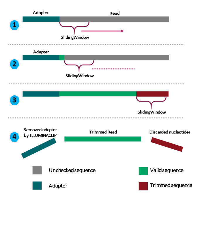
Figure 1: Source: https://carpentries-incubator.github.io/metagenomics/03-trimming-filtering/index.html
Additional resources for learning about Trimmomatic
https://www.genepattern.org/modules/docs/Trimmomatic/2/
Trimmomatic before genome assembly
FYI
Why are adapter sequences trimmed from only the 3' ends of reads?
We may also run FASTQC again after trimming to make sure that adapters have been removed and quality is good.
Tools for alignment
One of the challenges in analyzing high throughput sequencing is to reconstruct the genome of the unknown by using a knonw (ie. reference). The next step in analysis is to align our sequencing data to a reference genome. We used HISAT2 (splice aware) and visually compared the alignment results obtained from Bowtie2 (not splice aware) using the Integrative Genome Viewer (IGV). For RNA sequencing, we should use splice aware aligners to account for reads that map across two exons.
Obtaining expression read counts
After alignment of sequencing data to genome, we will need to count how many reads aligned to which gene. Using the tool featureCounts, we were able to do this. This tool takes as input our BAM alignment files and also an annotation file (gtf/gff) that tells us location of features (ie. genes, transcripts) in a genome. Note that for paired end sequencing we should include the additional flags below.
featureCounts version 2.0.1 (available on DNAnexus and Biostar environment on Biowulf)
-p: If specified, fragments (or templates) will be counted instead of reads. This option is only applicable for paired-end reads; single-end reads are always counted as reads.
featureCounts version 2.0.3 (default when using just Biowulf)
-p: Specify that input data contain paired-end reads. To perform fragment counting (ie. counting read pairs), the '--countReadPairs' parameter should also be specified in addition to this parameter.
--countReadPairs: Count read pairs (fragments) instead of reads. This option is only applicable for paired-end reads.
"For paired end reads, you should count read pairs (fragments) rather than reads because counting fragments will give you more accurate counts. There are several reasons why you cannot get the fragment counts by simply dividing the counts you got from counting reads by two. One reason is that a fragment with two mapped reads will give you two counts when you count reads, but a fragment with only one mapped read will only contribute one count (this fragment should get 1 count in fragment counting but it ended up with 0.5 count when you count reads instead of fragments). Another reason is that some reads may be found to be overlapping with more than one gene and therefore were not counted, but the corresponding fragments may be counted because the ambiguity was solved by longer fragment length." -- Wei Shi
Differential expression analysis
After obtaining the expression counts for each gene, we can run helper R scripts provided by the author of the Biostar Handbook to obtain differential gene expression results. In our lessons, we used deseq2.r. We also generated visualizations that show us how genes cluster by expression (heatmap) and how samples cluster together (PCA).
Learning objectives
An alternative to aligning raw sequencing data to a reference genome is to map them to a reference transcriptome. In this lesson, we will use the HBR and UHR datasets, and learn about this approach for analyzing RNA sequencing data and discuss some advantages and drawbacks. We will do the following
- Construct the human chromosome 22 reference transcriptome using FASTA file for the chromosome 22 reference genome and gtf file
- Align sequencing reads to the reference transcriptome
- Obtain differential expression
Before getting started, be sure to change into the ~/biostar_class/hbr_uhr directory.
cd ~/biostar_class/hbr_uhr
Constructing human chromosome 22 reference transcriptome
While we can always download reference genomes and reference transcriptomes from repositories such as NCBI or Ensembl, we will use gffread to create one from the chromosome 22 genome (22.fa) that we have used when analyzing the HBR and UHR data via alignment to the genome.
Make a reference transcriptome using gffread with the following options:
- -w tells gffread to write a FASTA file with sequences of all exons from a transcript, which is followed by the output file name (in this example, we are storing the reference transcriptome, 22_transcriptome.fa in the refs folder so we need to specify that path as well since we are currently in the ~/biostar_class/hbr_uhr folder)
- -W tells gffread to include the exon coordinates in the header of each sequence (ie. the sequencing header that starts with ">")
- -g prompts us to enter the reference genome FASTA file (22.fa in our case)
- the gtf (22.gtf) annotation file is provided at the end
gffread -w refs/22_transcriptome.fa -W -g refs/22.fa refs/22.gtf
Using head we can view the first few transcripts in human chromosome 22.
head refs/22_transcriptome.fa
Here, we can see that each transcript has a header line that starts with ">" followed by the actual sequence of the transcript. On the header line we have the transcript ID, which starts with ENST (they are from Ensembl) and genomic coordinates for the transcripts.
>ENST00000615943.1 loc:chr22|10736171-10736283|- exons:10736171-10736283 segs:1-113
ATCACTTCTCGGCCTTTTGGCTAAGATCAACTGTAGTATCTGTTGTTATTAATATAATATTGTATATTCA
ACCAATTGTCAATACAAGGCTGTTTGTATCTGATATGAACCAA
>ENST00000618365.1 loc:chr22|10936023-10936161|- exons:10936023-10936161 segs:1-139
AGCATGCCCAGTTAATTTGAAATTTCAGATAAACAAATACTTTTTTCAGTGTAAGTATATCCCATACAAT
ATTTGGGACATGCTTATACTAAAATATTATTCCTTATTTATCTGAAATTGAAATTTAACTGGGTATTAC
>ENST00000623473.1 loc:chr22|11065974-11067346|- exons:11065974-11066015,11067335-11067346 segs:1-12,13-54
GCTGCAGGCAGTGTTCTTCTGTGTCTGCTCACCGAGCTGCTCCGAGCCCGGCTT
>ENST00000624155.1 loc:chr22|11066501-11068089|+ exons:11066501-11066515,11067985-11068089 segs:1-15,16-120
ATGGCAGCCGGAGCGGTTTTTCTGGCATTGTCTGCCCAGCTGCTCCAAGCCAGACTGATGAAGGAGGAGT
Alignment of HBR and UHR raw sequencing data to human chromosome 22 transcriptome
Before we can align the HBR and UHR raw sequencing data to human chromosome 22 transcriptome, we need to create an index of this transcriptome (like we did with the genome). This will make the alignment proceed more efficiently. To do this we will use the index option of salmon where
- -t prompts us to input the FASTA file corresponding to the reference transcriptome (22_transcriptome.fa)
- -i prompts us to specify the name of a folder that will contain the indexing output
salmon index -t refs/22_transcriptome.fa -i refs/22_transcriptome.idx
Let's create a folder, salmon to store our alignment outputs with salmon
mkdir salmon
After the index has been generated, we can use salmon quant with the options below to generate our expression counts table. Below is how we would construct the command for one sample, however, we have 6 samples in the HBR and UHR dataset so we can turn to the parallel command to align all of these at the same time.
- -l prompts us to specify the library type and specifying "A" will allow salmon to automatically infer library type (ie. if the library is paired end)
- --validateMappings helps to make alignment more accurate
Selective alignment, first introduced by the --validateMappings flag in salmon, and now the default mapping strategy (in version 1.0.0 forward), is a major feature enhancement introduced in recent versions of salmon. When salmon is run with selective alignment, it adopts a considerably more sensitive scheme that we have developed for finding the potential mapping loci of a read... -- https://salmon.readthedocs.io/en/latest/salmon.html.
- For paired end sequencing, we specify read 1 and read 2 after the flags -1 and -2, respectively
- -o prompts us to specify a name of the folder where the output will be stored (we want our output to be stored in the folder salmon, which was created earlier)
salmon quant -i refs/22_transcriptome.idx -l A --validateMappings -1 reads/HBR_1_R1.fq -2 reads/HBR_1_R2.fq -o salmon/HBR_1_SALMON
Because we have 6 samples, we want to get Salmon to quantify them in one go so we will need to create a text file called ids.txt that contains the sample names for this dataset.
cd ~/biostar_class/hbr_uhr/reads
parallel echo {1}_{2} ::: HBR UHR ::: 1 2 3 > ids.txt
Now, go back up one directory to ~/biostar_class/hbr_uhr
cd ..
To align multiple files, we will use the following command
cat reads/ids.txt | parallel "salmon quant -i refs/22_transcriptome.idx -l A --validateMappings -1 reads/{}_R1.fq -2 reads/{}_R2.fq -o salmon/{}_SALMON"
Now if we change into the salmon directory and list the content, we should see the folders below, which contain the transcriptome alignment output for each sample in the HBR and UHR dataset (Salmon produces an output folder for each sample).
cd salmon
ls -1
HBR_1_SALMON
HBR_2_SALMON
HBR_3_SALMON
UHR_1_SALMON
UHR_2_SALMON
UHR_3_SALMON
Let's take a look at the contents of the HBR_1 alignment results folder.
cd HBR_1_SALMON
ls -1
aux_info
cmd_info.json
libParams
lib_format_counts.json
logs
quant.sf
If we need to recall how we ran the salmon alignment, we can see this in cmd_info.json, where cmd stands for command line (so this file provides command line information).
cat cmd_info.json
"salmon_version": "1.7.0",
"index": "22_transcriptome.idx",
"libType": "A",
"validateMappings": [],
"mates1": "HBR_1_R1.fq",
"mates2": "HBR_1_R2.fq",
"output": "salmon/HBR_1_SALMON",
"auxDir": "aux_info"
If we look at the salmon_quant.log file in the logs directory, we can get some information such as overall alignment rate.
cd logs
cat salmon_quant.log
Mapping rate = 34.6147%
The expression counts are available in the file quant.sf so to take a look at the HBR_1 Salmon quantifications we need to go up one folder (ie. ~/biostar_class/hbr_uhr/salmon/HBR_1_SALMON).
cd ..
Below, we use the column command to show the first few lines of column 4 in quant.sf file for HBR_1, which contains the count data.
- column is used to print our tabular data, which is quant.sf for HBR_1 nicely with columns aligned
- -t finds the number of columns in the data
- we use | to pipe the column output to sed, where
- 1q will print the first line of our table and then quit, preventing the first line from being included in the sort
- then we use sort where
- -k prompts us to specify the column we like to sort by (column 4 containing the count data in this case)
- we want to sort column 4 numerically so we use n after the 4 to indicate this
- we also want to sort column 4 from largest to smallest so we include r, with the final construct being "-k 4nr" for sorting column 4 numerically from largest to smallest
Hit q to get out of the column command and return to the prompt
column -t quant.sf | (sed 1q; sort -k 4nr) | head
The columns in the quant.sf Salmon output file are described below.
- Name: contains transcript IDs
- Length: transcript length (ie. number of bases in the transcript)
- EffectiveLength: the computed effective length of the target transcript. It takes into account all factors being modeled that will effect the probability of sampling fragments from this transcript, including the fragment length distribution and sequence-specific and gc-fragment bias (if they are being modeled) -- https://salmon.readthedocs.io/en/latest/file_formats.html
- TPM: this stands for Transcripts Per Million (these are normalized expression and we discussed normalization in the previous lesson). Here TPM is way to scale the library size or total number of counts per sample to one million (ie. for a given sample, how many reads will fall onto a particular gene if the total reads we have is one million?)
Name                Length  EffectiveLength  TPM            NumReads
ENST00000365188.1   283     116.921          123216.364027  282.000
ENST00000248975.5   1825    1651.938         29248.111343   945.757
ENST00000401609.5   1289    1115.938         16045.787239   350.501
ENST00000417718.6   569     395.946          12253.336005   94.968
ENST00000216146.8   1442    1268.938         11781.878918   292.646
ENST00000396680.2   1419    1245.938         11320.546468   276.091
ENST00000215909.9   560     386.946          9409.708625    71.271
ENST00000396821.7   4791    4617.938         9210.768077    832.591
ENST00000328933.9   4391    4217.938         8779.491093    724.866
Let's now change back in the ~/biostar_class/hbr_uhr/salmon folder
cd ~/biostar_class/hbr_uhr/salmon
We will next combine the expression for all of the HBR and UHR samples into one csv file. To do this, we need a design.csv file like we did with the alignment to genome analysis. As a review, the design file has two columns, where one column provides the sample names, and the other informs of the condition with which the samples were treated. Fortunately, the design file has been created already and they should be in the folder design_file_salmon in our home directory. For now, we want design.csv.
ls ~/design_file_salmon
design.csv
design.txt
To work with the design.csv file, we will need to copy it to the ~/biostar_class/hbr_uhr/ folder (so let's change into this)
cd ~/biostar_class/hbr_uhr/
cp ~/design_file_salmon/design.csv .
To view the contents of the design.csv file, we can use cat
cat design.csv
sample,condition
HBR_1_SALMON,HBR
HBR_2_SALMON,HBR
HBR_3_SALMON,HBR
UHR_1_SALMON,UHR
UHR_2_SALMON,UHR
UHR_3_SALMON,UHR
Note that the sample names in the design file matches the names of the salmon alignment output folders.
Now that we have the design file, run the combine_transcripts.r script to get a table with the expression for all samples. This script takes as input the design.csv file and the folder that contains the salmon output for all of the samples (ie. the salmon directory).
Rscript $CODE/combine_transcripts.r design.csv salmon
[1] "# Tool: Combine transcripts"
[1] "# Sample:  design.csv"
[1] "# Data dir:  salmon"
reading in files with read_tsv
1 2 3 4 5 6
[1] "# Results:  counts.csv
Below we show the first 4 lines of the merged salmon counts table, using the column command, where
- column is used to print tabular data nicely aligned in our terminal
- -t obtains the number of columns in our input file (which is counts.csv)
- -s allows us to specify the column separator, which is a "," because we are working with a csv or comma separated value file, where the columns in the file are separated by ","
- we use | to send the output from column to sed, where
- 1q will print the first line of our table and then quit, preventing the first line from being included in the sort
- then we use sort where
- -k prompts us to specify the column we like to sort by (column 2 the HBR_1 counts)
- we want to sort column 2 numerically so we use n after the 2 to indicate this
- we also want to sort column 2 from largest to smallest so we include r, with the final construct being "-k 2nr" for sorting column 2 numerically from largest to smallest
Hit q to get out of the column command and return to the prompt
column -t -s ',' counts.csv | (sed 1q; sort -k 2nr) | head -n 4
ensembl_transcript_id  HBR_1_SALMON  HBR_2_SALMON  HBR_3_SALMON  UHR_1_SALMON  UHR_2_SALMON  UHR_3_SALMON
ENST00000255882.10     1091.338      1127.926      986.09        326.662       275.629       287.17
ENST00000248975.5      945.757       1254.448      1141.565      237.221       191.815       286.847
ENST00000396821.7      832.591       994.288       903.553       1858.596      1181.578      1407.533
Obtaining differentially expressed genes
After the merged expression counts table has been created, we can proceed with differential expression analysis. Let's use DESeq2 again for this. But first, let's move counts.csv (the merged salmon expression table) to the folder salmon so we can keep all our salmon outputs in one place. Let's move the design.csv file as well.
mv counts.csv salmon/
mv design.csv salmon/
Change back into the salmon directory so we can run differential analysis.
cd salmon
Rscript $CODE/deseq2.r
converting counts to integer mode
estimating size factors
estimating dispersions
gene-wise dispersion estimates
mean-dispersion relationship
final dispersion estimates
fitting model and testing
[1] "# Tool: DESeq2"
[1] "# Design:  design.csv"
[1] "# Input:  counts.csv"
[1] "# Output:  results.csv"
As we seen previously, the deseq2.r script writes the differential analysis output to a file called results.csv. To view the differential analysis results let's do the following. Hit q to exit column and return to the prompt.
- column is used to print tabular data nicely aligned in our terminal
- -t obtains the number of columns in our input file (which is results.csv)
- -s allows us to specify the column separator, which is a "," because we are working with a csv or comma separated value file, where the columns in the file are separated by ","
column -t -s ',' results.csv | less -S
name                baseMean  baseMeanA  baseMeanB  foldChange   log2FoldChange  lfcSE  stat   PValue   PAdj     FDR     falsePos  HBR_1_SALMON  HBR_2_SALMON  HBR_3_SALMON
ENST00000390323.2   1182.9    0          2365.7     11306.612    13.5            1.62   8.33   7.9e-17  2.3e-13  0       0         0             0             0
ENST00000328933.9   480.4     939.3      21.6       0.023        -5.4            0.68   -8.01  1.2e-15  3.3e-12  0       0         876           1007.7        934.1
ENST00000390325.2   234.8     0          469.6      2244.479     11.1            1.62   6.86   7.1e-12  2.1e-08  0       0         0             0             0
ENST00000329492.5   203.7     399.9      7.5        0.019        -5.8            0.86   -6.68  2.5e-11  7.1e-08  0       0         377           411.8         411
ENST00000396425.7   431.4     822.7      40.2       0.049        -4.4            0.66   -6.63  3.4e-11  9.7e-08  0       0         810.7         789.6         867.7
ENST00000454349.6   145.8     291.6      0          0.001        -10.9           1.67   -6.54  6.3e-11  1.8e-07  0       0         188.5         383.1         303.3
Mapping transcript IDs to gene names
Note that we now have differential expression by transcripts and our first column contains the transcript IDs. But what genes do these transcripts map to? We will need to do some data wrangling to find out.
First let's sort the results.csv file by transcript ID and save it as results_id_sorted.txt to denote that this is a sorted version. To obtain the results_id_sorted.txt file, we
- use grep to find ENST, which is the prefix to the transcript ids in the results.csv file
- use | to send the grep results to column to generate a nicely aligned print out - note that in the column command, even though we use -s to specify that the columns in the input are comma separated, column will print the results to the terminal as a tab separated table
- use | to send the column output to sort
- finally, > save the sorted output as results_id_sorted.txt
grep ENST results.csv | column -t -s ',' | sort > results_id_sorted.txt
Next, we go back to the ~/biostar_class/hbr_uhr folder.
cd ~/biostar_class/hbr_uhr
We have the 22.gtf file that tells us the genes, transcripts, exons and other features that reside on human chromosome 22. There is tool called gtfToGenePred that can help us extract the transcripts and gene names from the gtf file.
We can pull up the documentation for gtfToGenePred if we just type "gtfToGenePred" in the command prompt.
gtfToGenePred - convert a GTF file to a genePred
usage:
   gtfToGenePred gtf genePred

options:
     -genePredExt - create a extended genePred, including frame
      information and gene name
     -allErrors - skip groups with errors rather than aborting.
      Useful for getting infomation about as many errors as possible.
     -ignoreGroupsWithoutExons - skip groups contain no exons rather than
      generate an error.
     -infoOut=file - write a file with information on each transcript
     -sourcePrefix=pre - only process entries where the source name has the
      specified prefix.  May be repeated.
     -impliedStopAfterCds - implied stop codon in after CDS
     -simple    - just check column validity, not hierarchy, resulting genePred may be damaged
     -geneNameAsName2 - if specified, use gene_name for the name2 field
      instead of gene_id.
     -includeVersion - it gene_version and/or transcript_version attributes exist, include the version
      in the corresponding identifiers.
If you remember in 22.gtf, under the attribute column we have things like gene id, gene name, etc (see the table below). We will use the option geneNameAsName2 to pull the gene names. We will also be using the genePredExt option to create the genePred file.
| CHROMOSOME | DATA SOURCE | FEATURE | START | END | SCORE | STRAND | FRAME | ATTRIBUTE |
|---|---|---|---|---|---|---|---|---|
| chr22 | ENSEMBL | gene | 10736171 | 10736283 | . | - | . | gene_id "ENSG00000277248.1"; gene_type "snRNA"; gene_status "NOVEL"; gene_name "U2"; level 3; |
| chr22 | ENSEMBL | transcript | 10736171 | 10736283 | . | - | . | gene_id "ENSG00000277248.1"; transcript_id "ENST00000615943.1"; gene_type "snRNA"; gene_status "NOVEL"; gene_name "U2"; transcript_type "snRNA"; transcript_status "NOVEL"; transcript_name "U2.14-201"; level 3; tag "basic"; transcript_support_level "NA"; |
| chr22 | ENSEMBL | exon | 10736171 | 10736283 | . | - | . | gene_id "ENSG00000277248.1"; transcript_id "ENST00000615943.1"; gene_type "snRNA"; gene_status "NOVEL"; gene_name "U2"; transcript_type "snRNA"; transcript_status "NOVEL"; transcript_name "U2.14-201"; exon_number 1; exon_id "ENSE00003736336.1"; level 3; tag "basic"; transcript_support_level "NA"; |
Here, we will use the genePredExt and geneNameAsName2 to get gene names included in our output.
Note that in the gtfToGenePred command below, we are saving the genePred output to the refs folder.
gtfToGenePred -genePredExt -geneNameAsName2 refs/22.gtf refs/22_extended.genePred
Taking a glance at the 22_extended.genePred file, we see that the first column has the transcript IDs, followed by strand and genomic coordinate information. The 12th column has the gene names. So columns 1 and 12 are what we want. The genePred format actually stands for gene prediction, which is exactly what it does, it tells us information abosut genes and their transcripts.
ENST00000615943.1  chr22  -  10736170  10736283  10736283  10736283  1  10736170,           10736283,           0  U2          none    none    -1,
ENST00000618365.1  chr22  -  10936022  10936161  10936161  10936161  1  10936022,           10936161,           0  CU459211.1  none    none    -1,
ENST00000623473.1  chr22  -  11065973  11067346  11065973  11067346  2  11065973,11067334,  11066015,11067346,  0  CU104787.1  incmpl  incmpl  0,0,
ENST00000624155.1  chr22  +  11066500  11068089  11066500  11068089  2  11066500,11067984,  11066515,11068089,  0  BAGE5       cmpl    cmpl    0,0,
ENST00000422332.1  chr22  +  11124336  11125705  11125705  11125705  2  11124336,11124507,  11124379,11125705,  0  ACTR3BP6    none    none    -1,-1,ENST00000612732.1  chr22  -  11249808  11249959  11249959  11249959  1  11249808,           11249959,           0  5_8S_rRNA   none    none    -1,
ENST00000614148.1  chr22  -  11253604  11253719  11253719  11253719  1  11253604,           11253719,           0  AC137488.1  none    none    -1,ENST00000614087.1  chr22  -  11275564  11275637  11275637  11275637  1  11275564,           11275637,           0  AC137488.2  none    none    -1,
ENST00000621672.1  chr22  +  11456855  11456937  11456937  11456937  1  11456855,           11456937,           0  CU013544.1  none    none    -1,ENST00000610677.1  chr22  -  11478157  11478241  11478241  11478241  1  11478157,           11478241,           0  CT867976.1  none    none    -1,
Here, we use cut to extract column 1 (transcript ID) and column 12 (gene name) of the genePred file and save it to 22_transcript_to_gene.txt.
cut -f1,12 refs/22_extended.genePred > refs/22_transcript_to_gene.txt
column -t refs/22_transcript_to_gene.txt | head
ENST00000615943.1   U2
ENST00000618365.1   CU459211.1
ENST00000623473.1   CU104787.1
ENST00000624155.1   BAGE5
ENST00000422332.1   ACTR3BP6
ENST00000612732.1   5_8S_rRNA
ENST00000614148.1   AC137488.1
ENST00000614087.1   AC137488.2
ENST00000621672.1   CU013544.1
Note that some genes may appear more than once because they can have multiple transcript products. As an example SLC25A17.
grep SLC25A17 refs/22_transcript_to_gene.txt
ENST00000263255.10  SLC25A17
ENST00000491545.5   SLC25A17
ENST00000435456.6   SLC25A17
ENST00000544408.5   SLC25A17
ENST00000402844.7   SLC25A17
ENST00000447566.5   SLC25A17
ENST00000420970.5   SLC25A17
ENST00000430221.5   SLC25A17
ENST00000427084.5   SLC25A17
ENST00000458600.5   SLC25A17
ENST00000443810.5   SLC25A17
ENST00000412879.5   SLC25A17
ENST00000426396.5   SLC25A17
ENST00000434193.5   SLC25A17
ENST00000478550.1   SLC25A17
ENST00000449676.5   SLC25A17
ENST00000434185.1   SLC25A17
Now let's sort 22_transcript_to_gene.txt, which contains our transcript ID to gene name mapping by transcript ID and save it as 22_transcript_to_gene_id_sorted.txt to denote that it is sorted.
cat refs/22_transcript_to_gene.txt | sort > refs/22_transcript_to_gene_id_sorted.txt
Finally, we can change back into the salmon output directory (cd salmon) to paste (the command that we will use is called paste) the sorted transcript ID to gene name mapping file (22_transcript_to_gene_id_sorted.txt) to the sorted differential expression analysis results (results_id_sorted.txt) and save as results_with_gene_names.txt.
cd salmon
The input for the paste command below are the two files that we want to paste together.
paste ../refs/22_transcript_to_gene_id_sorted.txt results_id_sorted.txt > results_with_gene_names.txt
Again, to view results_with_gene_names.txt we can use the column command (note that in the column command below, we did not specify the column separator because they are already separated by tabs)
column -t results_with_gene_names.txt | less -S
We should also insert column headers. To this use the sed command where inside the single quotes,"1i" tells it to insert into the first line the text that follows. Because results_with_gene_names.txt is tab separated, we would need to separate the column header by tabs using "\t" following each heading.
sed '1i TRANSCRIPT_NAME\tGENE_NAME\tTRANSCRIPT_ID\tbaseMean\tbaseMeanA\tbaseMeanB\tfoldChange\tlog2FoldChange\tlfcSE\tstat\tPValue\tPAdj\tFDR\tfalsePos\tHBR_1\tHBR_2\tHBR_3\tUHR_1\tUHR_2\tUHR_3' results_with_gene_names.txt > results_with_gene_names_labeled.txt
The sed command is known as a stream editor. It has many functions including printing of specific lines, deletion of lines, substitutions, and inserstion of lines.
Interpretation and comparison to alignment based RNA sequencing
Let's now take a look at our final differential analysis results table (results_with_gene_names_labeled.txt), using the SLC2A11 gene as an example and below we
- use the column command to print the contents of results_with_gene_names_labeled.txt nicely aligned in the terminal where -t finds out how many columns are in the input.
- use | to send the column output to sed where
- 1q prints the first line and quits
- then we grep to search for SLC2A11
- use | to send the output to another sed where
- 1q prints the first line and quits, thus preventing the first line from being sorted
- use -k to denote we want to sort by a specific column (column 8, which is log2FoldChange)
- n to sort column 8 numerically and r to sort from largest to smallest
- 1q prints the first line and quits, thus preventing the first line from being sorted
- less -S allows us to scroll through the table horizontally as well as vertically
column -t results_with_gene_names_labeled.txt | (sed 1q; grep SLC2A11) | (sed 1q; sort -k 8nr) | less -S
Below, we see the transcripts derived from SLC2A11. This is where classification based analysis is beneficial - it allows us to look at transcript level expression differences between conditions such that even though we are talking about the same gene, different transcript isoforms maybe expressed under different conditions or between tissue types. On the other hand, in alignment based analysis, we are aligning everything to the genome so we are getting aggregate gene level expression information.
TRANSCRIPT_NAME     GENE_NAME           TRANSCRIPT_ID       baseMean  baseMeanA  baseMeanB  foldChange   log2FoldChange  lfcSE  stat   PValue   PAdj     FDR     false
ENST00000611880.4   SLC2A11             ENST00000612482.4   12.5      0          25         119.482      6.9             1.89   3.64   2.7e-04  7.5e-01  0.0038  0
ENST00000418102.5   SLC2A11             ENST00000418170.5   11.9      0          23.7       113.292      6.8             2.75   2.48   1.3e-02  1.0e+00  0.0809  16
ENST00000403208.7   SLC2A11             ENST00000403222.7   3.3       0          6.7        31.867       5               3.92   1.27   2.0e-01  1.0e+00  0.4717  306
ENST00000473357.1   SLC2A11             ENST00000473487.6   2.6       0          5.1        24.428       4.6             3.92   1.18   2.4e-01  1.0e+00  0.5181  373
ENST00000423972.5   SLC2A11             ENST00000424008.1   0.6       0          1.3        6.022        2.6             3.94   0.66   5.1e-01  1.0e+00  NA      NA
ENST00000489322.5   SLC2A11             ENST00000489424.5   0.6       0          1.3        6.064        2.6             3.96   0.66   5.1e-01  1.0e+00  NA      NA
ENST00000482576.1   SLC2A11             ENST00000482652.1   7.2       2.6        11.7       4.435        2.1             1.31   1.64   1.0e-01  1.0e+00  0.3265  136
ENST00000436643.5   SLC2A11             ENST00000436663.1   0.3       0          0.6        2.693        1.4             4.04   0.35   7.2e-01  1.0e+00  NA      NA
ENST00000405847.5   SLC2A11             ENST00000405878.5   348.2     247.7      448.6      1.812        0.9             0.82   1.04   3.0e-01  1.0e+00  0.5981  499
ENST00000405286.6   SLC2A11             ENST00000405309.7   17.7      14.9       20.5       1.377        0.5             1.48   0.31   7.6e-01  1.0e+00  0.9274  2008
ENST00000255830.7   SLC2A11             ENST00000255830.7   0         0          0          NA           NA              NA     NA     NA       NA       NA      NA
ENST00000316185.8   SLC2A11             ENST00000316185.8   0         0          0          NA           NA              NA     NA     NA       NA       NA      NA
ENST00000440493.5   SLC2A11             ENST00000440562.1   0         0          0          NA           NA              NA     NA     NA       NA       NA      NA
ENST00000461809.5   SLC2A11             ENST00000461833.1   0         0          0          NA           NA              NA     NA     NA       NA       NA      NA
ENST00000467660.5   SLC2A11             ENST00000467672.5   0         0          0          NA           NA              NA     NA     NA       NA       NA      NA
ENST00000472526.1   SLC2A11             ENST00000472575.5   0         0          0          NA           NA              NA     NA     NA       NA       NA      NA
ENST00000492516.1   SLC2A11             ENST00000492538.1   0         0          0          NA           NA              NA     NA     NA       NA       NA      NA
ENST00000405340.6   SLC2A11             ENST00000405409.6   460.8     634.9      286.6      0.451        -1.1            0.61   -1.89  5.9e-02  1.0e+00  0.2441  77
ENST00000473740.5   SLC2A11             ENST00000473782.1   0.2       0.4        0          0.372        -1.4            4.08   -0.35  7.3e-01  1.0e+00  NA      NA
ENST00000486907.1   SLC2A11             ENST00000487165.5   5.6       8.4        2.9        0.343        -1.5            2.11   -0.73  4.6e-01  1.0e+00  0.7522  930
ENST00000491948.5   SLC2A11             ENST00000491967.1   1.6       2.4        0.9        0.366        -1.5            2.24   -0.65  5.2e-01  1.0e+00  NA      NA
ENST00000345044.10  SLC2A11             ENST00000345044.10  19        30.1       7.8        0.258        -2              1.46   -1.34  1.8e-01  1.0e+00  0.4439  263
A drawback to the classification based approach is that we are mapping to a known database of transcripts. This may prevent us from discovering expression of novel splice isoforms.
Visualizing gene expression
Let's now create a gene expression heatmap for results generated using the classification based approach. We have our results.csv and design.csv file in our salmon directory so we just need to do the following to create the heatmap.
Rscript $CODE/create_heatmap.r
To view the heatmap, copy it to the ~/public directory.
cp heatmap.pdf ~/public/hbr_uhr_heatmap_salmon.pdf
To generate the PCA plot, we need a tab separated version of the design file, which we can copy over from ~/biostar_class/design_file_salmon folder. Since we are in ~/biostar_class/hbr_uhr/salmon we can use "." to denote copy to here, our present working directory.
cp ~/design_file_salmon/design.txt .
Let's use cat to view design.txt. Again, the difference between design.csv and design.txt is that the columns are separated by commas in the csv file and by tabs in the txt file.
cat design.txt
sample  condition
HBR_1_SALMON    HBR
HBR_2_SALMON    HBR
HBR_3_SALMON    HBR
UHR_1_SALMON    UHR
UHR_2_SALMON    UHR
UHR_3_SALMON    UHR
To generate the PCA plot, we will also need a tab separated version of the counts table, which we can generate using the code below where
- cat is used to print contents of a file (ie. counts.csv)
- tr is used to replace commas (denoted by ',') in this file with tabs (denoted by '\t')
cat counts.csv | tr ',' '\t' > counts.txt
Then, we run the create_pca.r script like we did with the alignment based analysis method.
Rscript $CODE/create_pca.r counts.txt design.txt 6
To view the pca, copy it to the public directory.
cp pca.pdf ~/public/hbr_uhr_pca_salmon.pdf